- Page 2 and 3:
Aerothermochemistry Gregorio Millá
- Page 4 and 5:
PRESENTACIÓN Amable Liñán Es un
- Page 6 and 7:
que no cambiaron los resultados, y
- Page 8:
INSTITUTO NACIONAL DE TÉCNICA AERO
- Page 11 and 12:
aim to become acquainted with Aerot
- Page 13 and 14:
Tarifa, Manuel de Sendagorta and Ig
- Page 15 and 16:
3.4 Energy equation . . . . . . . .
- Page 17 and 18:
8.4 Quenching . . . . . . . . . . .
- Page 20 and 21:
Chapter 1 Thermochemistry 1.1 Intro
- Page 22 and 23:
1.1. INTRODUCTION 3 GAS ε/k (K) σ
- Page 24 and 25:
1.1. INTRODUCTION 5 14 12 10 N 2 CH
- Page 26 and 27:
1.2. THERMODYNAMIC FUNCTIONS OF AN
- Page 28 and 29:
1.2. THERMODYNAMIC FUNCTIONS OF AN
- Page 30 and 31:
1.3. MIXTURE OF GASES 11 Helmholtz
- Page 32 and 33:
1.3. MIXTURE OF GASES 13 is the par
- Page 34 and 35:
1.3. MIXTURE OF GASES 15 Entropy Si
- Page 36 and 37:
1.4. CALCULATION OF THE THERMODYNAM
- Page 38 and 39:
1.4. CALCULATION OF THE THERMODYNAM
- Page 40 and 41:
1.5. CHEMICAL REACTIONS IN A MIXTUR
- Page 42 and 43:
1.6. CHEMICAL EQUILIBRIUM 23 Since
- Page 44 and 45:
∆G 0 j = ∑ i 1.7. CASE OF A MIX
- Page 46 and 47:
1.7. CASE OF A MIXTURE OF IDEAL GAS
- Page 48 and 49:
1.8. CHEMICAL KINETICS 29 1.8 Chemi
- Page 50 and 51:
1.8. CHEMICAL KINETICS 31 Mechanics
- Page 52 and 53:
1.8. CHEMICAL KINETICS 33 This stru
- Page 54 and 55:
1.8. CHEMICAL KINETICS 35 [3] Hirsc
- Page 56 and 57:
Chapter 2 Transport phenomena in ga
- Page 58 and 59:
2.2. DIFFUSION 39 Hereinafter, nota
- Page 60 and 61:
2.2. DIFFUSION 41 where r is the di
- Page 62 and 63:
2.2. DIFFUSION 43 T ∗ Ω (1,1)∗
- Page 64 and 65:
2.2. DIFFUSION 45 Gas Pair σ 12 (
- Page 66 and 67:
2.2. DIFFUSION 47 coefficients. 14
- Page 68 and 69:
2.3. VISCOSITIES 49 2.3 Viscosities
- Page 70 and 71:
2.3. VISCOSITIES 51 Here µ and µ
- Page 72 and 73:
2.3. VISCOSITIES 53 Its value depen
- Page 74 and 75:
2.4. THERMAL CONDUCTIVITY 55 2000 1
- Page 76 and 77:
2.4. THERMAL CONDUCTIVITY 57 4000 3
- Page 78 and 79:
Chapter 3 General equations 3.1 Int
- Page 80 and 81:
3.2. EQUATION OF CONTINUITY 61 The
- Page 82 and 83:
3.2. EQUATION OF CONTINUITY 63 A i
- Page 84 and 85:
3.4. ENERGY EQUATION 65 where the s
- Page 86 and 87:
3.4. ENERGY EQUATION 67 The energy
- Page 88 and 89:
3.5. GENERAL EQUATIONS 69 obtained
- Page 90 and 91:
3.6. ENTROPY VARIATION 71 Taking in
- Page 92 and 93:
3.7. ONE-DIMENSIONAL MOTIONS 73 red
- Page 94 and 95:
3.8. STATIONARY, ONE-DIMENSIONAL MO
- Page 96 and 97:
3.9. THE CASE OF ONLY TWO CHEMICAL
- Page 98 and 99:
3.10. STATIONARY, ONE-DIMENSIONAL M
- Page 100 and 101:
3.10. STATIONARY, ONE-DIMENSIONAL M
- Page 102 and 103:
3.10. STATIONARY, ONE-DIMENSIONAL M
- Page 104 and 105:
3.11. APPENDIX: NOTATION AND REPERT
- Page 106 and 107:
3.11. APPENDIX: NOTATION AND REPERT
- Page 108 and 109:
Chapter 4 Combustion Waves 4.1 Deto
- Page 110 and 111:
4.2. KINDS OF DETONATIONS AND DEFLA
- Page 112 and 113:
4.2. KINDS OF DETONATIONS AND DEFLA
- Page 114 and 115:
4.3. VELOCITY OF THE BURNT GASES 95
- Page 116 and 117:
4.3. VELOCITY OF THE BURNT GASES 97
- Page 118 and 119:
4.4. PROPAGATION VELOCITY 99 p H’
- Page 120 and 121:
4.5. APPLICATIONS 101 By substituti
- Page 122 and 123:
4.7. INDETERMINACY OF THE SOLUTION
- Page 124 and 125:
Chapter 5 Structure of the combusti
- Page 126 and 127: 5.2. WAVE EQUATIONS 107 of diffusio
- Page 128 and 129: 5.2. WAVE EQUATIONS 109 2) Burnt ga
- Page 130 and 131: 5.4. LIMITING FORM OF THE WAVE EQUA
- Page 132 and 133: 5.4. LIMITING FORM OF THE WAVE EQUA
- Page 134 and 135: 5.5. DETONATIONS 115 Of these two v
- Page 136 and 137: 5.5. DETONATIONS 117 waves. Such th
- Page 138 and 139: 5.5. DETONATIONS 119 This relation
- Page 140 and 141: 5.5. DETONATIONS 121 curves, repres
- Page 142 and 143: 5.6. DEFLAGRATIONS 123 mum temperat
- Page 144 and 145: 5.6. DEFLAGRATIONS 125 8 7 v/v 1 =T
- Page 146 and 147: 5.7. TRANSITION FROM DEFLAGRATION T
- Page 148 and 149: 5.7. TRANSITION FROM DEFLAGRATION T
- Page 150 and 151: Chapter 6 Laminar flames 6.1 Introd
- Page 152 and 153: 6.1. INTRODUCTION 133 papers presen
- Page 154 and 155: 6.3. BOUNDARY CONDITIONS 135 c) Dif
- Page 156 and 157: 6.4. MODIFICATION OF THE CONDITIONS
- Page 158 and 159: 6.4. MODIFICATION OF THE CONDITIONS
- Page 160 and 161: 6.6. EXAMPLE 141 generally impossib
- Page 162 and 163: 6.6. EXAMPLE 143 Two more relations
- Page 164 and 165: 6.7. REACTION VELOCITY 145 1.0 0.8
- Page 166 and 167: 6.8. FLAME EQUATIONS 147 6.8 Flame
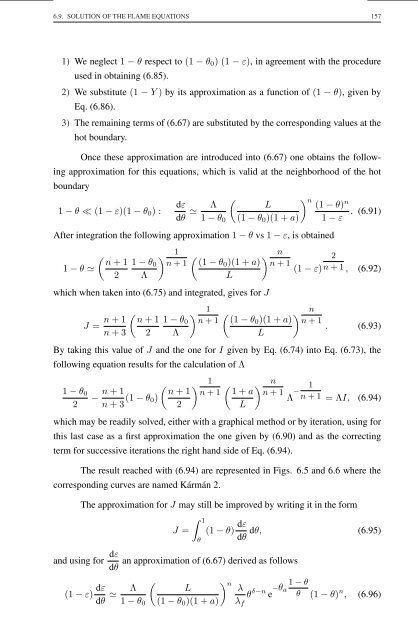
- Page 168 and 169: 6.9. SOLUTION OF THE FLAME EQUATION
- Page 170 and 171: 6.9. SOLUTION OF THE FLAME EQUATION
- Page 172 and 173: 6.9. SOLUTION OF THE FLAME EQUATION
- Page 174 and 175: 6.9. SOLUTION OF THE FLAME EQUATION
- Page 178 and 179: 6.10. STRUCTURE OF THE COMBUSTION W
- Page 180 and 181: 6.11. IGNITION TEMPERATURE 161 6.11
- Page 182 and 183: 6.12. GENERAL EQUATIONS FOR THE COM
- Page 184 and 185: 6.12. GENERAL EQUATIONS FOR THE COM
- Page 186 and 187: 6.12. GENERAL EQUATIONS FOR THE COM
- Page 188 and 189: 6.13. OZONE DECOMPOSITION FLAME 169
- Page 190 and 191: 6.13. OZONE DECOMPOSITION FLAME 171
- Page 192 and 193: 6.13. OZONE DECOMPOSITION FLAME 173
- Page 194 and 195: 6.13. OZONE DECOMPOSITION FLAME 175
- Page 196 and 197: 6.14. HYDRAZINE DECOMPOSITION FLAME
- Page 198 and 199: 6.14. HYDRAZINE DECOMPOSITION FLAME
- Page 200 and 201: 6.14. HYDRAZINE DECOMPOSITION FLAME
- Page 202 and 203: 6.14. HYDRAZINE DECOMPOSITION FLAME
- Page 204 and 205: 6.14. HYDRAZINE DECOMPOSITION FLAME
- Page 206 and 207: 6.15. FLAME PROPAGATION IN HYDROGEN
- Page 208 and 209: 6.15. FLAME PROPAGATION IN HYDROGEN
- Page 210 and 211: 6.15. FLAME PROPAGATION IN HYDROGEN
- Page 212 and 213: 6.15. FLAME PROPAGATION IN HYDROGEN
- Page 214 and 215: 6.15. FLAME PROPAGATION IN HYDROGEN
- Page 216 and 217: 6.15. FLAME PROPAGATION IN HYDROGEN
- Page 218 and 219: 6.15. FLAME PROPAGATION IN HYDROGEN
- Page 220 and 221: 6.15. FLAME PROPAGATION IN HYDROGEN
- Page 222 and 223: 6.15. FLAME PROPAGATION IN HYDROGEN
- Page 224 and 225: 6.15. FLAME PROPAGATION IN HYDROGEN
- Page 226 and 227:
Chapter 7 Turbulent flames 7.1 Intr
- Page 228 and 229:
7.1. INTRODUCTION 209 300 250 TURBU
- Page 230 and 231:
7.2. TURBULENT COMBUSTION THEORIES
- Page 232 and 233:
7.2. TURBULENT COMBUSTION THEORIES
- Page 234 and 235:
7.2. TURBULENT COMBUSTION THEORIES
- Page 236 and 237:
7.2. TURBULENT COMBUSTION THEORIES
- Page 238 and 239:
7.4. COMPARISON WITH EXPERIMENTAL R
- Page 240 and 241:
Chapter 8 Ignition, flammability an
- Page 242 and 243:
8.2. IGNITION 223 comparison betwee
- Page 244 and 245:
8.3. FLAMMABILITY LIMITS 225 The pr
- Page 246 and 247:
8.4. QUENCHING 227 8.4 Quenching So
- Page 248 and 249:
8.4. QUENCHING 229 [19] Simon, D. M
- Page 250 and 251:
Chapter 9 Flows with combustion wav
- Page 252 and 253:
9.2. CONDITIONS THAT MUST BE SATISF
- Page 254 and 255:
9.3. NORMAL FLAME FRONT 235 9.3 Nor
- Page 256 and 257:
9.4. INCLINED FLAME FRONT 237 60 50
- Page 258 and 259:
9.5. ENTROPY JUMP ACROSS THE FLAME
- Page 260 and 261:
9.5. ENTROPY JUMP ACROSS THE FLAME
- Page 262 and 263:
9.6. VORTICITY ACROSS THE FLAME 243
- Page 264 and 265:
Chapter 10 Aerothermodynamic field
- Page 266 and 267:
10.1. INTRODUCTION 247 form numeric
- Page 268 and 269:
10.1. INTRODUCTION 249 ∆ P /∆ P
- Page 270 and 271:
10.2. TSIEN METHOD 251 As aforesaid
- Page 272 and 273:
10.2. TSIEN METHOD 253 1.0 λ=6.0 M
- Page 274 and 275:
10.3. METHOD OF FABRI-SIESTRUNCK-FO
- Page 276 and 277:
10.3. METHOD OF FABRI-SIESTRUNCK-FO
- Page 278 and 279:
10.5. CHAMBER WITH SLOWLY VARYING C
- Page 280 and 281:
Chapter 11 Similarity in combustion
- Page 282 and 283:
11.2. DIMENSIONLESS PARAMETERS OF A
- Page 284 and 285:
11.2. DIMENSIONLESS PARAMETERS OF A
- Page 286 and 287:
11.3. SCALING OF ROCKETS 267 Furthe
- Page 288 and 289:
11.3. SCALING OF ROCKETS 269 From h
- Page 290 and 291:
11.4. SCALING OF ROCKETS FOR NON-ST
- Page 292 and 293:
11.4. SCALING OF ROCKETS FOR NON-ST
- Page 294 and 295:
11.5. FLAME STABILIZATION 275 Flame
- Page 296 and 297:
11.5. FLAME STABILIZATION 277 Flame
- Page 298 and 299:
11.5. FLAME STABILIZATION 279 which
- Page 300 and 301:
Chapter 12 Diffusion flames 12.1 In
- Page 302 and 303:
12.1. INTRODUCTION 283 In fact, oth
- Page 304 and 305:
12.1. INTRODUCTION 285 which preced
- Page 306 and 307:
12.1. INTRODUCTION 287 remains appr
- Page 308 and 309:
12.2. GENERAL EQUATIONS FOR LAMINAR
- Page 310 and 311:
12.3. BOUNDARY CONDITIONS ON THE FL
- Page 312 and 313:
12.4. SIMPLIFIED EQUATIONS 293 As f
- Page 314 and 315:
12.4. SIMPLIFIED EQUATIONS 295 whil
- Page 316 and 317:
12.5. SOLUTIONS OF THE SIMPLIFIED S
- Page 318 and 319:
12.5. SOLUTIONS OF THE SIMPLIFIED S
- Page 320 and 321:
Chapter 13 Combustion of liquid fue
- Page 322 and 323:
13.2. ATOMIZATION 303 lem has been
- Page 324 and 325:
13.4. COMBUSTION 305 solution corre
- Page 326 and 327:
13.5. NOTATION 307 2) The phenomeno
- Page 328 and 329:
13.6. CONTINUITY EQUATIONS 309 Chem
- Page 330 and 331:
13.7. ENERGY EQUATION 311 The value
- Page 332 and 333:
13.8. DIFFUSION EQUATIONS 313 13.8
- Page 334 and 335:
13.9. COMBUSTION VELOCITY OF THE DR
- Page 336 and 337:
13.10. INTEGRATION OF THE EQUATIONS
- Page 338 and 339:
13.11. NUMERICAL APPLICATION 319 wh
- Page 340 and 341:
13.11. NUMERICAL APPLICATION 321 10
- Page 342 and 343:
13.12. COMPARISON WITH EXPERIMENTAL
- Page 344 and 345:
13.14. COMBUSTION OF FUEL SPRAYS 32
- Page 346 and 347:
13.15. DROPLET EVAPORATION 327 4 0.
- Page 348 and 349:
13.15. DROPLET EVAPORATION 329 1 0.
- Page 350 and 351:
13.16. APPENDIX: APPLICATION OF PRO
- Page 352 and 353:
13.16. APPENDIX: APPLICATION OF PRO
- Page 354 and 355:
13.16. APPENDIX: APPLICATION OF PRO