Daniel l. Rubinfeld

258 Part 2 Producers, Consumers, and Competitive Markets
Marginal, average, and total
cost are discussed in §7.2.
Price
(dollars per
unit)
60
50
-40
30
20
10
o
0
C
The choice of the profit-maximizing output by a competitiye firm is so impor_
tant that we will devote most of the rest of this chapter to analyzing it We begin
with the short-run output decision and then move to the long run.
HOlY much output should a finn produce over the short run, when the firm's
plant size is fixed In this section we show how a firm can use information about
revenue and cost to make a profit-maximizing output decision.
'10
M &
2 3 5
Lost profit for
111 < '1*
&ii&¥
6 7 8
'1*
Lost profit for
'72 > '1*
=~=== AR = ::v1R = p
ATC
AVC
9 10 11
Output
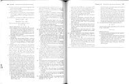
In the short run, the competitive firm maximizes its profit by choosing an output 1]* at which its marginal cost MCis:.
to the P (or marginal revenue MR) of its product. The profit of the firm is measured by the rectangle;
Profit is maximized at point A, where output is q* = 8 and the price is $40,
because marginal reven:le is e~u~l. to marginal cost at this point. To see that
* =:= 8 is indeed the proht-maxlmlzmg output, note that at a 10l\'er output, say
q =:= 7, marginal revenue is greater than marginal cost; profit could thus be
i~creased by increasing output. The shaded area between 1]1 = 7 and q* shows
the lost profit associated with producing at 1]1' At a higher output, say ib mar­
"inal cost is greater than marginal revenue; thus, reducing output saves a cost
tl1at exceeds the reduction in revenue. The shaded area between q* and 1]2 = 9
shoWS the lost profit associated 'with producing at ih
The MR and MC curves cross at an output of qo as well as q*. At qo, however,
profit is clearly not maximized. An increase in output beyond qo increases profit
because marginal cost is ,veIl belOlY marginal revenue. We can thus state the
condition for profit maximization as follows: MargiJl(zl revenue equals lIlarginal
cost at a poillt at wlziclz tlze I/wrgillal cost Cllrue is rising. This conclusion is very
important because it applies to the output decisions of firms in markets that may
or may not be perfectly competitive. We can restate it as follows:
Output Rule: If a firm is producing any output at all, it should produce at the
level at 'which marginal revenue equals marginal cost.
The Short-Run
a Competitive Firm
Figure 8.3 also shows the competitive firm's short-run profit. The distance AB is
the difference between price and average cost at the output level q*, which is the
average profit per unit of output. Segment BC measures the total number of
units produced. Rectangle ABCD, therefore, is the firm's profit.
A firm need not always earn a profit in the short run, as Figure 8.4 shows.
The major difference from Figure 8.3 is a higher fixed cost of production. This
higher fixed cost raises average total cost but does not change the average variable
cost and marginal cost curves. At the profit-maximizing output q*, the price P is
less than average cost. Line segment AB, therefore, measures the average loss
from production. Likevvise, the rectangle ABCD now measures the firm's total loss.
IVhy doesn't a firm that earns a loss leave an industry entirely A firm might
operate at a loss ill tlze slzort rllil because it expects to earn a profit in the fuhue,
when the price of its product increases or the cost of production falls, and
because shutting down and starting up again would be costly. In fact, a finn has
two choices in the short run: It can produce some output, or it can shut down
production temporarily. It will compare the profitability of producing with the
profitability of shutting down and choose the preferred outcome. If the price of the
product is greater tlzan the aI1ernge ecollomic cost of production, tlze finll makes a positive
economic profit by producillg. Consequelltly, it-will choose to produce.
But suppose that the price is less than average total cost, as shown in Figure
8.4. If it continues to produce, the firm minimizes its losses at output q*. Note
that in Figure 8.4, because of the presence of fixed costs, average variable cost is
less than average total cost and the firm is indeed losing money. The firm should
~erefore consider shutting down. If it does, it earns no revenue, but it avoids the
fixed as well as variable cost of production. If there are no sunk costs so that
average economic cost is equal to average total cost, the firm should indeed shut
down. Because there are no sunk costs, it can invest its capital elsewhere or, for
that matter, reenter the industry if and when economic conditions improve.
To summarize: When there are no sunk costs, the firm's average total cost is
eqal to its average economic cost Thus, tlze firm should shut dowll when the price
of Its product is less thall tlze average total cost at tlze profit-Illaximizillg output.
8 Profit Maximization and Competitive Supply 259