Daniel l. Rubinfeld

m
54 Part Introduction: Markets and Prices
The government, however, has decided that Po is too high and mandated that
the price can be no higher than a maximum allo'wable ceiling price, denoted by
P max' What is the result At this lower price, producers (particularly those with
hiaher costs) will produce less, and the quantity supplied will drop to Q1' Consu~ers,
on the other hand, will demand more at this 1m\' price; they would like
to purchase the quantity Q2' Demand therefore exceeds supply, and a shortage
develops-i.e., there is excess dellland. The amount of excess demand is Q2 Q1'
This excess demand sometimes takes the form of queues, as 'when drivers
lined up to buy gasoline during the winter of 1974 and the summer of 1979. In
both instances, the lines were the result of price controls; the government prevented
domestic oil and gasoline prices from rising along 'with 'world oil prices.
Sometimes excess demand results in curtailments and supply rationing, as with
nahual gas price controls and the resulting gas shortages of the mid-1970s, wh~r:
industrial consumers closed factories because gas supplies were cut ott.
Sometimes it spills over into other markets, 'where it artificially increases
demand. For example, natural gas price controls caused potential buyers of gas
to use oil instead.
Some people gain and some lose from price controls. As Figure 2.22 suggests,
producers lose: They receive lower prices, and some leave the industry. Some but
not all consumers gain. While those who can purchase the good at a lower price
are better off, those who have been "rationed out" and carmot buy the good at all
are worse off. How large are the gains to the winners and hO'vv large are the losses
to the losers Do total gains exceed total losses To ans\·ver these questions we
need a method to measure the gains and losses from price controls and other
forms of government intervention. We discuss such a method in Chapter 9.
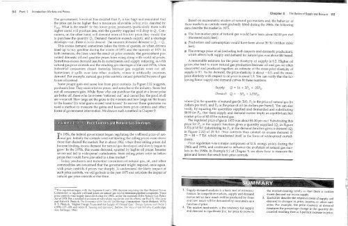
In 1954, the federal government began regulating the wellhead price of natural
gas. Initially the conh'ols were not binding; the ceiling prices were above
those that cleared the market. But in about 1962, when these ceiling prices did
become binding, excess demand for nahiral gas developed and slowly began to
grow. In the 1970s, this excess demand, spurred by higher oil prices, became
severe and led to widespread curtailments. Soon ceiling prices were far below
prices that would have prevailed in a free market. 15
Today, producers and industrial consumers of natural gas, oil, and other
commodities are concerned that the government might respond, once again,
with price controls if prices rise sharply. To understand the likely impact of
such price controls, we will go back to the year 1975 and calculate the impact of
natural gas price conh'ols at that time.
Based on econometric shidies of natural gas markets and the behavior of
those markets as controls were gradually lifted during the 1980s, the follOWing
data describe the market in 1975.
TI1e free-market price of natural gas would have been about $2.00 per mef
(thousand cubic feet);
Production and consumption would have been about 20 Tef (trillion cubic
feet);
The average price of oil (including both imports and domestic production),
which affects both supply and demand for natural gas, was about $8/barrel.
A reasonable estimate for the price elasticity of supply is 0.2. Higher oil
prices also lead to more natural gas production because oil and gas are often
discovered and produced together; an estimate of the cross-price elasticity of
supply is 0.1. As for demand, the price elasticity is about 0.5, and the crossprice
elasticity with respect to oil price is about 1.5. You can verify that the following
linear supply and demand curves fit these numbers:
Sllpply:
Q = 14 + 2P c + .25P o
Demand: Q = 5Pc + 3.75P o ,
where Q is the quantity of natural gas (in Tef), Pc is the price of natural gas (in
dollars per mef), and Po is the price of oil (in dollars per barrel). You can also
verify, by equating the quantities supplied and demanded and substituting
$8.00 for Po, that these supply and demand curves imply an equilibrium free
market price of $2.00 for natural gas.
The regulated price of gas in 1975 was about $1.00 per mcf. Substituting this
price for Pc in the supply function gives a quantity supplied (Q1 in Figure
2.22) of 18 Tef. Substituting for P G in the demand function gives a demand (Q2
in Figure 2.22) of 25 Tct Price controls thus created an excess demand of
25 - 18 = 7 Tef, which manifested itself in the form of widespread curtailments.
Price regulation was a major component of U.s. energy policy during the
1960s and 1970s, and continued to influence the evolution of natural gas markets
in the 1980s. In Example 9.1 of Chapter 9, we show how to measure the
gains and losses that result from price controls.
~h .. n·t"',. 2 The Basics of Supply and Demand 55
15 This reo-ulation beo-an with the Supreme Court's 1954 decision requiring the then Federal Power
Commission to reo-ulate wellhead prices on nahrral aas sold to interstate pipeline companies. These
00.
price controls were largely remo\'ed during the 1980s, under the mandate of the NahrralGas PolIc\'
Act of 1978 .. For a detailed discussion of natural gas regulation and its effects, see Paul IV. MacA\'oy
and Robert S. Pind\,ck, The Ecollolllics ofthe 0Jntul'Ill Gns Shortage (Amsterdam: North-Holland, 1975);
R S. Pindyck, "Higher Energy Prices imd the Supply of Natural G.as," Energy Systellls nnd Policy 2
(1978): 177-209; and Arlon R Tussing and Cormie C Barlow, The Natlil'lll GIlS Industnl (Cambndge,
MA: Ballinger, 1984)
1. Supply-demand analysis is a basic tool of microeconomics.
In competitive markets, supply and demand
curves tell us how much will be produced by firms
and how much will be demanded by consumers as a
function of price.
2. The market mechanism is the tendency for supply
and demand to equilibrate (Le., for price to move to
the market-clearing level), so that there is neither
excess demand nor excess supply.
3. Elasticities describe the responsiveness of supply and
demand to changes in price, income, or other variables.
For example, the price elasticity of demand
measures the percentage change in the quantity demanded
resulting from a I-percent increase in price,