Daniel l. Rubinfeld
Daniel l. Rubinfeld
Daniel l. Rubinfeld

You also want an ePaper? Increase the reach of your titles
YUMPU automatically turns print PDFs into web optimized ePapers that Google loves.
44 Part 1 Introduction: Markets and Prices<br />
In the intermediate run-say, one year after the freeze-both supply and<br />
demand are more elastic, supply because existing trees can be harvested more<br />
intensively (with some decrease in quality), and demand because consumers<br />
have had time to change their buying habits. As part (b) shows, although the<br />
intermediate-run supply curve also shifts to the left, price has come down from<br />
P 1 to P 2 . The quantity supplied has also increased somewhat from the short<br />
run, from Q1 to Q2' In the long run shown in part (c), price returns to its normal<br />
level because growers have had time to replace trees damaged by the freeze.<br />
TIle long-run supply curve, then, simply reflects the cost of producing coffee,<br />
including the costs of land, of planting and caring for the trees, and of a competitive<br />
rate of profit. 9<br />
Let's begin with the linear curves shown in Figure 2.1S. We can write these<br />
curves algebraically as follows:<br />
Demand: Q a - bP<br />
Supply:<br />
Q = c + dP<br />
2 The Basics of Supply and Demand 45<br />
(2.4a)<br />
(2.4b)<br />
Our problem is to choose numbers for the constants a, b, c, and d. This is done,<br />
for supply and for demand, in a two-step procedure:<br />
II Step 1: Recall that each price elasticity, whether of supply or demand, can be<br />
written as<br />
E<br />
(P/Q)(flQ/flP),<br />
*2.8<br />
So far our discussion of supply and demand has been largely qualitative. To use<br />
supply and demand curves to analyze and predict the effects of changing market<br />
conditions, we must begin attaching numbers to them. For example, to see<br />
how a 50-percent reduction in the supply of Brazilian coffee may affect the<br />
world price of coffee, we must determine actual supply and demand curves and<br />
then calculate the shifts in those curves and the resulting changes in price.<br />
In this section, we will see how to do simple ''back of the envelope" calculations<br />
with linear supply and demand curves. Although they are often approximations<br />
of more complex curves, we use linear curves because they are easier to work<br />
with. It may come as a surprise, but one can do some informative economic<br />
analyses on the back of a small envelope with a pencil and a pocket calculator.<br />
First, we must learn how to "fit" linear demand and supply curves to market<br />
data. (By this we do not mean statistical fitting in the sense of linear regression or<br />
other statistical techniques, which we discuss later in the book.) Suppose we<br />
have two sets of numbers for a particular market: The first set consists of the<br />
price and quantity that generally prevail in the market (i.e., the price and quantity<br />
that prevail" on average," when the market is in equilibrium, or when market<br />
conditions are "normal"). We call these numbers the equilibrium price and<br />
quantity and denote them by P* and Q*. The second set consists of the price elasticities<br />
of supply and demand for the market (at or near the equilibrium), which<br />
we denote by and ED, as before.<br />
These numbers may come from a statistical study done by someone else; they<br />
may be numbers that we simply think are reasonable; or they may be numbers<br />
that we want to tryout on a "what if" basis. Our goal is to write down the supply<br />
and demand curves that fit (i.e., are consistent with) these numbers. We can then<br />
determine numerically how a change in a variable such as GNP, the price of<br />
another good, or some cost of production will cause supply or demand to shift<br />
and thereby affect market price and quantity.<br />
9 You can learn more about the world coffee market from the Foreign Agriculture Service of the Us.<br />
Department of Agriculture. Their Web site is \\<br />
rLlrktet.htmL<br />
where flQ/flP is the change in quantity demanded or supplied resulting from<br />
a small change in price. For linear curves, liQ/liP is constant. From equations<br />
(2.4a) and (2.4b), we see that liQ/liP = d for supply and liQ/liP = b for<br />
demand. Now, let's substitute these values for liQ/liP into the elasticity formula:<br />
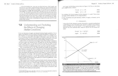
Price<br />
Dellland: Eo = b(P*/Q*)<br />
Supply:<br />
Es = d(P*/Q*),<br />
Q* a<br />
Q=a bP<br />
Quantity<br />
(2.5a)<br />
(2.5b)<br />
Linear supply and demand curves provide a convenient tool for analysis. Given data<br />
for the equilibrium price and quantity P* and Q*, as well as estimates of the elasticities<br />
of demand and supply ED and Es, we can calculate the parameters c and d for the<br />
supply curve and a and b for the demand curve. (In the case dravvn here, C < 0.) The<br />
curves can then be used to the behavior of the market