Daniel l. Rubinfeld

More documents

Recommendations

Info

106 Part 2 Producers, Consumers, and Competitive Markets 4 Individual and Market Demand curve D 2 . The upward-sloping income-consumption curve implies that an increase in income causes a shift to the right in the demand curve-in this case from D1 to D2 to D 3· Income (dollars per 30 month) &i& :¥&ii § In §2.3, we explain that the income elasticity of demand is the percentage change in the quantity demanded resulting from a I-percent increase in income. Engel curve Curve relating the quantity of a good consumed to income. Normal versus When the income-consumption curve has a positive slope, the quantity demanded increases with income. As a result, the income elasticity of demand is positive. The greater the shifts to the right of the demand curve, the larger the income elasticity. In this case, the goods are described as normal: Consumers want to buy more of them as their income increases. In some cases, the quantity demanded falls as income increases; the income elasticity of demand is negative. We then describe the good as inferior. The term inferior simply means that consumption falls when income rises. Hamburger, for example, is inferior for some people: As their income increases, they buy less hamburger and more steak. Figure 4.3 shows the income-consumption curve for an inferior good. For relatively low levels of income, both hamburger and steak are normal goods. As income rises, however, the income-consumption curve bends backward (from point B to C). This shift occurs because hamburger has become an inferior good-its consumption has fallen as income has increased. Engel Curves Income-consumption curves can be used to construct Engel curves, which relate the quantity of a good consumed to an individual's income. Figure 4.4 shows 15 Steak (units per month) 10 ... _ Income-Conswnption Curve 20 10, ~---~----~----~------~o Income (dollars per 30 month) 20 10 o Engel Curye 4 8 5 (a) (b) 12 16 Food (units per month) ] In'''''' 1 N"m~ T 10 Hamburger (units per month) Engel curves relate the quantity of a good consumed to income. In (a), food is a normal good and the Engel curve is upward sloping. In (b), however, hamburger is a normal good for income less than $20 per month and an inferior good for income greater than $20 month. 5 5 10 20 30 Hamburger (units per month) An increase in a person's income can lead to less consumption of one of the hvo goods being purchased. Here, hamburger, though a normal good behveen A and B, becomes an inferior good when the income-consumption curve bends backward behveen B and C. how such curves are constructed for rno different goods. Figure 4.4(a), which shows an upward-sloping Engel curve, is derived directly from Figure 4.2(a). In both figures, as the individual's income increases from $10 to $20 to $30, her consumption of food increases from 4 to 10 to 16 units. Recall that in Figure 4.2(a) the vertical axis measured lmits of clothing consumed per month and the horizontal axis units of food per month; changes in income were reflected as shifts in the budget line. In Figures 4.4(a) and (b), we have replotted the data to put income on the vertical axis \'.'hile keeping food and hamburger on the horizontal. The upward-sloping Engel curve in Figure 4.4(a)-like the upward-sloping income-consumption curve in Figure 4.2(a)-applies to all normal goods. Note that an Engel curve for clothing would have a similar shape (clothing consumption increases from 3 to 5 to 7 urlits as income increases).
108 Part 2 Producers, Consumers, and Competitive Markets 4 Individual and Market Demand Figure 4.4(b), derived from Figure 4.3, shows the Engel curve for hamburger. We see that hamburger consumption increases from 5 to 10 units as income increases from $10 to $20. As income increases further, from $20 to $30, consumption falls to 8 units. The portion of the Engel curve that slopes downward is the income range in which hamburger is an inferior good. '"' -¥ .-\nnual 580,000 Income 70,000 60,000 W55iw0§ii§ x 50,000 The Engel curves we just examined apply to individual consumers. However, we can also derive Engel curves for groups of consumers. This information is particularly useful if we want to see how consumer spending varies among different income groups. Table 4.1 illush'ates these spending patterns for several items taken from a survey by the U.s. Bureau of Labor Statistics. Although the data are averaged over many households, they can be interpreted as describing the expenditures of a typical family. Note that the data relate expenditures on a particular item rather than the q1lantity of the item to income. The first two items, entertainment and owned dwellings, are consumption goods for which the income elasticity of demand is high. Average family expendihlres on entertainment increase almost eightfold when we move from the lowest to highest income group. The same pattern applies to the purchase of homes: There is a more than tenfold increase in expenditures from the lowest to the highest category. In contrast, expenditures on rental housing actually fall with income. This pattern reflects the fact that most higher-income individuals own rather than rent homes. Thus rental housing is an inferior good, at least for incomes above $30,000 per year. Finally, note that health care, food, and clothing are consumption items for which the income elasticities are positive, but not as high as for entertainment or owner-occupied housing. 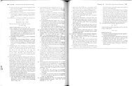The data Ul Table 4.1 have been plotted in Figure 4.5 for rented dwellings, health care, and entertainment. Observe in the three Engel curves that as .. ±O,OOO 30,000 20,000 10,000 ° SO 500 1,000 1,500 2,000 2,500 3,000 3,500 4,000 4,500 5,000 Annual Expenditure Average per-capita expenditures on rented dwellulgs, health care, and entertainment are plotted as functions of illU1ual income, Health care and entertainment are superior goods: Expenditures increase with income, Rental housing, however, is an inferior good for incomes above $30,000. &% income rises, expenditures on entertainment increase rapidly while expenditures on rental housing increase when uKome is low, but decrease once income exceeds 530,000. Substitutes and Complements EXPENDITURES ($) ON: Entertainment Owned dwellings Rented dwellings Health care Food Clothing INCOME GROUP (1997 $) LESS THAN 10,000- 20,000- 30,000- 40,000- 50,000- 70,000 10,000 19,000 29,000 39,000 49,000 69,000 AND ABOVE 700 947 1,274 1,514 2,054 2,654 4,300 1,116 1,725 2,253 3,243 4,454 5,793 9,898 1,957 2,170 2,371 2,536 2,137 1,540 1,266 1,031 1,697 1,918 1,820 2,052 2,214 2,642 2,656 3,385 4,109 4,888 5,429 6,220 8,279 859 978 1,363 1,772 1,778 2,614 3,442 Source: u.s. Department of Labor, Bureau of Labor Statistics, "Consumer Expenditure Survey: 1997." The demand curves that we graphed in Chapter 2 showed the relationship between the price of a good and the quantity demanded, vvith preferences, income, and the prices of all other goods held constant. For many goods, demand is related to the consumption and prices of other goods. Baseball bats and baseballs, hot dogs and mustard, and computer hardware and software are all examples of goods that tend to be used together. Other goods, such as cola and diet cola, owner-occupied houses and rental aparhnents, movie tickets and videocassette rentals, tend to substitute for one another. Recall from Section 2.4 that two goods are substitutes if an increase in the price of one leads to an increase in the quantity demanded of the other. If the price of a movie ticket rises, \'\'e would expect individuals to rent more videos, because mo\'ie tickets and videos are substitutes. Similarly, hvo goods are cOlllplelllents if an increase in the price of one good leads to a decrease in the quantity demanded of the other. If the price of gasoline goes up, causulg gasoline consumption to fall, we would expect the consumption of motor oil to fall as well, because gasoline and motor oil are used together. Two goods are illdepelldellt if a change in the price of one good has no effect on the quantity demanded of the other.
Page 1 and 2:
0-13-016583-2 TOO
Page 3 and 4:
Iii Iii iii Iii Iii Iii Iii Iii Iii
Page 5 and 6:
PART 1 Introduction: Marl
Page 7 and 8:
x Contents Contents xi 2 Producers
Page 9 and 10:
xiv Contents Contents 3 9.2 111e Ef
Page 11 and 12:
- Contents Contents 17 18 16.4 Effi
Page 13 and 14:
F xxii Contents Example 17.3 Reduci
Page 15 and 16:
--.. -~---.--.. '~~~~~~-~----------
Page 17 and 18:
PART 1 surveys the scope of microec
Page 19 and 20: 4 Part '1 Introduction: Markets and
Page 21 and 22: 8 Part 1 Introduction: Markets and
Page 25 and 26: 16 Part 'I Introduction: Markets an
Page 33 and 34: 32 Part 1 Introduction. Markets and
Page 35 and 36: 36 Part '1 Introduction Markets and
Page 47 and 48: few years ago, General Mills decide
Page 49 and 50: 64 Part 2 Producers, Consumers, and
Page 53 and 54: 72 Part '2 Producers, Consumers, an
Page 65 and 66: --------~ 96 Part 2 Producers, Cons
Page 67 and 68: 100 Part 2 Producers, Consumers, an
Page 69: 104 Part 2 Producers, Consumers, an
Page 85 and 86: 1136 Part 2 Producers, Consumers, a
Page 87 and 88: Part 2 Producers, Consumers, and Co
Page 89 and 90: 144 Part:2 Producers, Consumers, an
Page 91 and 92: - O far, we have assumed that price
Page 103 and 104: 1172 Part 2 Producers, Consumers, a
Page 121 and 122:
5 :; 208 Part 2 Producers, Consumer
Page 123 and 124:
$ 212 Part 2 Producers, Consumers,
Page 125 and 126:
216 Part 2 Producers, Consumers, an
Page 127 and 128:
Page 129 and 130:
Page 131 and 132:
Page 133 and 134:
Page 135 and 136:
Page 137 and 138:
Page 139 and 140:
Page 141 and 142:
Page 143 and 144:
Page 145 and 146:
Page 147 and 148:
Page 149 and 150:
Page 151 and 152:
Page 153 and 154:
Page 155 and 156:
Page 157 and 158:
Page 159 and 160:
Page 161 and 162:
Page 163 and 164:
292 Part:2 Producers, Consumers, an
Page 165 and 166:
Page 167 and 168:
Page 169 and 170:
Page 171 and 172:
Page 173 and 174:
Page 175 and 176:
Page 177 and 178:
Page 179 and 180:
F PART 3 examines a broad range of
Page 181 and 182:
I I n a perfectly competitive marke
Page 183 and 184:
Price Dollars per 7 I Unit of Outpu
Page 185 and 186:
334 Part 3 Market Structure and Com
Page 187 and 188:
Page 189 and 190:
Page 191 and 192:
Page 193 and 194:
Page 195 and 196:
Page 197 and 198:
Page 199 and 200:
show all

Daniel l. Rubinfeld

Create successful ePaper yourself

Delete template?

Save as template?