Daniel l. Rubinfeld

More documents

Recommendations

Info

266 Part 2 Producers, Consumers, and Competitive Markets illustrated by Figure 8.8 the first capacity constraint comes into effect whe producti~n reaches about 9700 barrels a day. A second capacity constrain~ becom:s .lmportant when production increases beyond 10,700 barrels a day. DeCldmg hovv much output to produce now becomes relati\'ely easy. Suppose that refined products can be sold for $23 per barrel. Because the marginal cost of production is close to $24 for the first unit of output, no crude oil should be run through the refinery at a price of $23. If, hmve\'er, price is between $24 and $25, the refinery should produce 9700 barrels a day (filling the thermal cracker). Finally, if the price is above $25, the more expensive refinincr mut should be used and production expanded toward 10,700 barrels a day. I) Because the cost function rises in steps, you know that your productio~ dea ~ions ne~~ not change much in response to slIlall changes in price. You will typ_ lcally uhllze sufficient crude oil to fill the appropriate processing unit until price increases (or decreases) substantially. In that case, you need simply calculate whether the increased price warrants using an additional, more expensive processing unit. = per unit 8 Profit Maximization and Competitive Supply 267 P3 ----------~-------.-------$------------------------------- I ; ; I I I I I I I I I I I I Po I I I ----~----~--$ : AF====~============~~ I I I I I I I I I I ~ ----,-----,--~--- I I I I I I I I I I I I I I I I I I I I I: 2 -± 5 7 8 10 15 21 Quantity 5 The short-rIm II/arket sllpply ellrve shows the am01.mt of output that the industry will produce in the short run for every possible price. The industry's output is the sum of the quantities supplied by all of its individual firms. Therefore, the market supply curve can be obtained by adding the supply curves of each of these firms. Figure 8.9 shows how this is done when there are only three firms all of which have different short-rill1 production costs. Each firm's ~arginal cos~ curve is drawn only for the portion that lies above its average variable cost curve. (We have shown only three finns to keep the graph simple, but the same analysis applies when there are many firms.) At any price below P1' the industry ,·vill produce no output because P 1 is the minimum average variable cost of the lowest-cost firm. Between P 1 and Pz, only firm 3 will produce. The industry supply curve, therefore, will be identical to that portion of firm 3's marginal cost curve Me 3 . At price Pz, the industry supply will be the sum of the quantity supplied by all three firms. Firm 1 supplies 2 units, firm 2 supplies 5 units, and firm 3 supplies 8 units. Industry supply is thus 15 units. At price P 3 , firm 1 supplies 4 units, firm 2 supplies 7 units, and firm 3 supplies 10 units; the industry supplies 21 units. Note that the industry supply curve is upward sloping but has a kink at price P 2 , the Im·vest price at which all tlu'ee firms produce. With many firms in the market, however, the kink becomes unimportant. Thus we usually draw industry supply as a smooth! upward-sloping curve. Elasticity of Market Supply Unfortunately, finding the industry supply curve is not ahvays as simple a5 adding up a set of individual supply curves. As price rises, all firms in the indush')' expand their output. This additional output increases the demand for inputs The short-run industry supply curve is the swmnation of the supply curves of the individual firms. Because the third firm has a lower ~verage variable cost cl~Te ~han the first two firms, the market supply curve S begins at price P 1 and follow~ the I~argmal cost c~rve of th~ t~d firm Me 3 until price equals P 2 , where there is a kink. For P2 and all prices above It, the mdustry quantity supplied IS the sum of the quantities supplied by each of the three firms. =-$ to production and may lead to higher input prices .. As we saw in Figure 8.7, increasing input prices shifts the finns' marginal cost curves upward. For example, an increased demand for beef could also increase demand for com and soybeans (which are used to feed cattle) and thereby cause the prices of these crops to rise. In turn, the higher input prices ,vould cause firms' marginal cost curves to shift upward. This increase lowers each firm's output choice (for any o-iven market price) and causes the industry supply cun"e to be less respOl~si~Te to changes in output price than it would otherwise be. The price elasticity of market supply measures the sensitivity of industry out ~ut to ma~'ket price. The elasticity of supply E, is the percentage change in quantity supphed Q in response to a I-percent change in price P: Beca.use marginal cost curves are up,·vard sloping, the short-nUl elasticity of supply IS always positive. When marginal costs increase rapidly in response to mcreas~s in output, the elasticity of supply is 10\,\'. Firms are then capacity ~onstrall1ed and find it costly to increase output But when marginal costs m~rease slowly in response to increases in output, supply is relatively elastic; in thIS case, a small price increase induces firms to produce much more . . At one extreme is the case of pelfeetly inelastic SllppiJ/, which arises when the md~stry's plant and equipment are so fully utilized tl;at greater output can be achIeved only if new plants are built (as they will be in the long run). At the other extreme is the case of pelfeetly elastic supply, which arises when marginal costs are constant. In §2.3, we define the elasticity of supply as the percentage change in quantity supplied resulting from a I-percent increase in price.
268 Part 2 Producers, Consumers, and Competitive Markets 8 Profit Maximization and Competitive Supply 269 I n the short run, the shape of the market supply curve for a mineral such as copper depends on how the cost of mining varies within and among the world's major producers. Costs of mining, smelting, and refining copper differ because of differences in labor and h'ansportation costs and because of differ_ ences in the copper content of the ore. Table 8.1 summarizes some of the relevant cost and production data for the nine largest copper-producing nations.4 These ~ata Cill1 be used to plot the ,:orld supply ~u~ve fo~' copper, The supply curve IS a short-run curve because It takes the eXisting mmes and refineries as fixed. Figure 8.10 shows how this curve is consh'ucted for the nine countries listed in the table. The complete world supply curve would, of course, incorporate data for all copper-producing cOlUltries. Note also that the curve in Figure 8.10 is an approximation. The marginal cost number for each country is an average for all copper producers in that COurltry. In the United States, for example, some producers have a marginal cost greater than 70 cents and some less. The lowest-cost copper is mined in Chile and Russia, where the marginal cost of refined copper is about 50 cents per pound. 5 The line segment labeled MCc, MC R represents the marginal cost curve for these counh·ies. The curve is horizontal until the total capacity to mine and refine copper for these hvo countries is reached. (That point is reached at a production level of about 4 million metric tons per year.) The line segment MC I , MCz describes the marginal cost curve for Indonesia and Zambia (where the marginal cost is about 55 cents per pound). Likewise, line segment MC A represents the marginal cost curve for Australia, and so on. 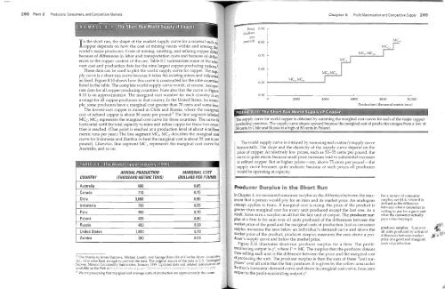ANNUAL PRODUCTION MARGINAL COST COUNTRY (THOUSAND METRIC TONS) (DOLLARS PER POUND) Price (dollars per pound) 0.80 0..70 0.60 050 OAO o 2000 4000 6000 8000 10,000 Production (thousand metric tons) The supply curve for world is obtained by summing the marginal cost curves for each of the major copperproducing cow1tries. The cwve slopes upward because the marginal cost of production ranges from a low of 50 cents in Chile and Russia to a of 80 cents in Poland. The vvodd supply curve is obtained by summing each nation's supply curve horizontally. The slope and the elasticity of the supply curve depend on the price of copper. At relatively low prices, such as 50-55 cents per pound, the curve is quite elastic because small price increases lead to substantial increases in refined copper. But at higher prices-say, above 75 cents pel' pound-the supply curve becomes quite inelastic because at such prices all producers would be operating at capacity. Australia 600 0.65 Canada 710 0.75 Chile 3,660 0.50 Indonesia 750 0.55 Peru 450 0.70 Poland 420 0.80 Russia 450 0.50 United States 1,850 0.70 Zambia 280 0.55 J Our thanks to James Burrows, Michael Loreth, and George Rainville of Charles River Associates, Inc, who were kind enough to provide the data. The original source of the data is US. Geological Survey, Mineral Commodity Summaries, January 1999 .. Updated data and related information are available on the \"1eb at htip:!/rnincrzd~< Irninera:::l/pub:-:/(OrnIl1odit:\, 5 We are presuming that marginal and average costs of production are approximately the same. Producer Surplus in Short In Chapter 4, vve measured consumer surplus as the difference between the maximum that a person would pay for an item and its market price. An analogous concept applies to firms. If marginal cost is rising, the price of the product is greater than marginal cost for e\'ery unit produced except the last one. As a result, firms earn a surplus on all but the last unit of output. The producer surplus of a firm is the sum over all units produced of the differences between the market price of the good and the marginal costs of production. Just as consumer surplus measures the area below an individual's demand curve and above the market price of the product, producer surplus measures the area abo\'e a producer's supply CUl've and below the market price. Figure 8.11 illustrates short-run producer surplus for a finn. The profitmaximizing output is q*, where P = Me. The surplus that the producer obtains frm selling each unit is the difference bet\'\'een the price and the marginal cost ot producing the unit. The producer surplus is then the sum of these "unit surpluses" over alllmits that the firm produces. It is aiven bv the vellow area under the firm's horizontal demand curve and above its ~nargir;al co;t curve, from zero output to the profit-maximizing output q*. For a review of consumer surplus, see §4A, where it is defined as the difference behveen what a consumer is willing to pay for a good and what the consumer actually pays when buying it producer surplus Sum over all units produced by a firm of differences behveen market price of a good and marginal costs of production.
Page 1 and 2:
0-13-016583-2 TOO
Page 3 and 4:
Iii Iii iii Iii Iii Iii Iii Iii Iii
Page 5 and 6:
PART 1 Introduction: Marl
Page 7 and 8:
x Contents Contents xi 2 Producers
Page 9 and 10:
xiv Contents Contents 3 9.2 111e Ef
Page 11 and 12:
- Contents Contents 17 18 16.4 Effi
Page 13 and 14:
F xxii Contents Example 17.3 Reduci
Page 15 and 16:
--.. -~---.--.. '~~~~~~-~----------
Page 17 and 18:
PART 1 surveys the scope of microec
Page 19 and 20:
4 Part '1 Introduction: Markets and
Page 21 and 22:
8 Part 1 Introduction: Markets and
Page 23 and 24:
Page 25 and 26:
16 Part 'I Introduction: Markets an
Page 27 and 28:
Page 29 and 30:
Page 31 and 32:
Page 33 and 34:
32 Part 1 Introduction. Markets and
Page 35 and 36:
36 Part '1 Introduction Markets and
Page 37 and 38:
Page 39 and 40:
Page 41 and 42:
Page 43 and 44:
Page 45 and 46:
Page 47 and 48:
few years ago, General Mills decide
Page 49 and 50:
64 Part 2 Producers, Consumers, and
Page 51 and 52:
Page 53 and 54:
72 Part '2 Producers, Consumers, an
Page 55 and 56:
Page 57 and 58:
Page 59 and 60:
Page 61 and 62:
Page 63 and 64:
Page 65 and 66:
--------~ 96 Part 2 Producers, Cons
Page 67 and 68:
100 Part 2 Producers, Consumers, an
Page 69 and 70:
Page 71 and 72:
Page 73 and 74:
Page 75 and 76:
Page 77 and 78:
Page 79 and 80:
Page 81 and 82:
Page 83 and 84:
Page 85 and 86:
1136 Part 2 Producers, Consumers, a
Page 87 and 88:
Part 2 Producers, Consumers, and Co
Page 89 and 90:
144 Part:2 Producers, Consumers, an
Page 91 and 92:
- O far, we have assumed that price
Page 93 and 94:
Page 95 and 96:
Page 97 and 98:
160 Part:2 Producers, Consumers, an
Page 99 and 100: 164 Part 2 Producers, Consumers, an
Page 103 and 104: 1172 Part 2 Producers, Consumers, a
Page 107 and 108: 180 Part:2 Producers, Consumers, an
Page 111 and 112: 88 Part 2 Producers, Consumers, and
Page 121 and 122: 5 :; 208 Part 2 Producers, Consumer
Page 123 and 124: $ 212 Part 2 Producers, Consumers,
Page 149: 264 Part 2 Producers, Consumers, an
Page 179 and 180: F PART 3 examines a broad range of
Page 181 and 182: I I n a perfectly competitive marke
Page 183 and 184: Price Dollars per 7 I Unit of Outpu
Page 185 and 186: 334 Part 3 Market Structure and Com
show all

Daniel l. Rubinfeld

You also want an ePaper? Increase the reach of your titles

Delete template?

Save as template?