Daniel l. Rubinfeld

More documents

Recommendations

Info

102 Part:2 Producers, Consumers, and Competitive Markets Individual and Market Demand depends on the demands of other people. These effects playa crucial role in the demands for many high-tech products, such as computer hardware and soft-vvare, and telecommunications systems. 6. Finally, we will briefly describe some of the methods that economists use to obtain empirical information about demand. x#= Clothing (units per month) #& A ; §!Ei In §3.3, we explain how consumers choose the market basket on the highest indifference curve that touches the consumer's budget line. In §3.2, we explain how the budget line shifts in response to a price change. price-consumption curve Curve tracing the utilitymaximizing combinations of two goods as the price of one changes. This section shows how the demand curve of an individual consumer follows from the consumption choices that a person makes when faced with a budget constraint. To illustrate these concepts graphically, we will limit the available goods to food and clothing and vdll rely on the utility-maximization approach described in Section 3.3. Price Changes We begin by examining ways in which the consumption of food and clothing changes when the price of food changes. Figure 4.1 shows the consumption choices that a person '\-"ill make when allocating a fixed amount of income between the nvo goods. Initially, the price of food is 51, the price of clothing $2, and the consumer's income $20. The utility-maximizing consumption choice is at point B in Figure 4.1(a). Here, the consumer buys 12 units of food and 4 units of clothing, thus achieving the level of utility associated with indifference curve U 2 • Now look at Figure 4.1(b), which shows the relationship between the price of food and the quantity demanded. The horizontal axis measures the quantity of food consumed, as in Figure 4.1(a), but the vertical axis now measures the price of food. Point G in Figure 4.1(b) corresponds to point B in Figure 4.1(a). At G, the price of food is $1, and the consumer purchases 12 units of food. Suppose the price of food increases to 52. As we saw in Chapter 3, the budget line in Figure 4.1(a) rotates inward about the vertical intercept, becoming n"ice as steep as before. The higher relative price of food has increased the magnitude of the slope of the budget line. The consumer now achieves maximum utility at A, which is found on a lower indifference curve, U 1 . (Because the price of food has risen, the consumer's purchasing power-and thus attainable utility-has fallen.) At A, the consumer chooses 4 units of food and 6 units of clothing. In Figure 4.1(b), this modified consumption choice is at E, which shows that at a price of $2, 4 units of food are demanded. Finally, ,\,,'hat will happen if the price of food deCl'eases to 50 cents Because the budget line now rotates outward, the consumer can achieve the higher level of utility associated with indifference CUD'e U 3 in Figure 4.1(a) by selecting D, 'with 20 units of food and 5 units of clothing. Point H in Figure 4.1(b) shows the price of 50 cents and the quantity demanded of 20 units of food. The Individual Demand Curve We can go on to include all possible changes in the price of food. In Figure 4.1(a), the price-consumption curve traces the utility-maximizing combinations of food and clothing associated with every possible price of food. Note that as the price of food falls, attainable utility increases and the consumer buys more food. 6 -:~A 5 4 Price of Food 52,00 150 LOO 50 r' I -, I _..1 __ I I I I I I I I I :4 :12 :20 I I I I I (a) I I I I I I I : I I --F : : I I I I I I I I I I I I I I I I : I I I : : I I i _+ ____ ~G I : :1 : I ",;II I I', ! H -,------;-----, I I I I I I I I I : I I 4 12 20 (b) Price-Consumption Curve Food (units per month) Demand Curve Food (units per month) A reduction in the price of food, with income and the price of clothing fixed, causes this consumer to choose a different market basket. In (a), the baskets that maximize utility for various prices of food (point A, $2; B, $1; D, $0.50) trace out the priceconsumption curve. Part (b) gives the demand curve, which relates the price of food to the demanded. (Points E, G, and H correspond to points A, B, and D, resl)ectiv This pattern of increasing consumption of a good in response to a decrease in price almost always holds. But '\'\'hat happens to the consumption of clothing as the price of food falls As Figure 4.1(a) shows, the consumption of clothing may either increase or decrease. Both food and clothing consumption can increase because the decrease in the price of food has increased the consumer's ability to purchase both goods. An individual demand curve relates the quantity of a good that a single con Sumer will buy to the price of that good. In Figure 4.1(b), the individual demand Curve relates the quantity of food that the consumer will buy to the price of food. This demand curve has h-vo important properties. individual demand curve Curve relating the quantity of a good that a single consumer will buy to its price.,
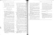
104 Part 2 Producers, Consumers, and Competitive Markets Chapter 4 Individual and Market Demand 105 In §3.1, we introduce the marginal rate of substitution as a measure of the maximum amount of one good that the consumer is willing to give up in order to obtain one unit of another good .. 1. The level of utility that call be attailled changes as we mO've alo1lg the curve. The lower' the price of the product, the higher its level of utility. Note from Figure 4.1(a) that a higher indifference cun'e is reached as the price falls. Again, this result simply reflects the fact that as the price of a product falls, the consumer's purchasing power increases. 2. At every poillt 011 the demalld curve, the cOllsumer is maximizillg utility by satisfyi1lg the c01lditioll that the margi1lal rate of substitutioll (MRS) of food for clothing equals the ratio of the prices of food a1ld clothillg. As the price of food falls, the price ratio and the MRS also fall. In Figure 4.1, the price ratio falls from 1 (52/52) at E (because the Cl.lrv'e U j is tangent to a budget line with a slope of -1 at A) to 1/2 ($1/$2) at G, to 1/4 ($050/$2) at H. Because the consumer is maximizing utility, the MRS of food for clothing decreases as we move down the demand CUlTe. This phenomenon makes intuitive sense because it tells us that the relative value of food falls as the consumer buys more of it. M i %§§%£ w Clothing (units per month) 7 5 3 &&Ai Income-Consumption Curve LI3 Food (units per month) ¥¥ The fact that the MRS varies along the indiv'idual's demand CUIye tells us something about how consumers value the consumption of a good or service. Suppose we were to ask a consumer hm\' much she would be willing to pay for an additional milt of food ,>vhen she is currently consLUning 4 milts. Point E on the demand curve in Figure 4.l(b) provides the answer: $2. Why As we pointed out above, because the MRS of food for clothing is 1 at E, one additional unit of food is worth one additional lmit of clothing. But a unit of clothing costs $2, \'\'ruch is, therefore, the value (or marginal benefit) obtained by consuming an additionalmut of food. Thus, as we move dmvn the demand curve in Figure 4.1(b), the MRS falls. Likewise, the value that the consumer places on an additional milt of food falls from $2 to $1 to S0.50. Price of Food $1.00 D2 D3 Income Changes We have seen what happens to the consumption of food and clothing when the price of food changes. Now let's see what happens when income changes. The effects of a change in income can be analyzed in much the same way as a price change. Figure 4.2(a) shows the consumption choices that a consumer will make when allocating a fixed income to food and clothing when the price of food is $1 and the price of clothing $2. As in Figure 4.l(a), the quantity of clothing is measured on the vertical axis and the quantity of food on the horizontal axis. Income changes appear as changes in the budget line. Initially, the consumer's income is S10. The utility-maximizing consumption choice is then at A, at vvhich she buys 4 units of food and 3 units of clothing. This choice of 4 units of food is also shown in Figure 4.2(b) as E on demand CUITe OJ. Demand curve OJ is the curve that would be traced out if we held income fixed at $10 but uaried the price offood. Because we are holding the price of food constant, we will observe only a single point E on this demand curve. What happens if the consumer's income is increased to $20 Her budget line then shifts outward parallel to the original budget line, allowing her to attain the utility level associated with indifference curve U 2 . Her optimal consumption choice is now at B, 'where she buys 10 units of food and 5 units of clothing. In Figure 4.2(b) her consumption of food is shown as G on demand curve O 2 , O 2 is the demand curve that would be traced out if we held income fixed at $20 but varied the price of food. Finally, note that if her income increases to $30, she chooses 0, with a market basket containing 16 units of food (and 7 units of clothing), represented by H in Figure 4.2(b). 4 10 16 (b) Food (units per month) An increase in income, with the prices of all goods fixed, causes consumers to alter their choices of market basket. In part (a), the baskets that maximize consumer satisfaction for various incomes (point A, $10; B, $20; D, $30) trace out the incomeconsumption curve. The shift to the right of the demand curve in response to the increases in income is shown in part (b). (Points E, G, and H correspond to points A, B, and 0, r'P
Page 1 and 2:
0-13-016583-2 TOO
Page 3 and 4:
Iii Iii iii Iii Iii Iii Iii Iii Iii
Page 5 and 6:
PART 1 Introduction: Marl
Page 7 and 8:
x Contents Contents xi 2 Producers
Page 9 and 10:
xiv Contents Contents 3 9.2 111e Ef
Page 11 and 12:
- Contents Contents 17 18 16.4 Effi
Page 13 and 14:
F xxii Contents Example 17.3 Reduci
Page 15 and 16:
--.. -~---.--.. '~~~~~~-~----------
Page 17 and 18: PART 1 surveys the scope of microec
Page 19 and 20: 4 Part '1 Introduction: Markets and
Page 21 and 22: 8 Part 1 Introduction: Markets and
Page 25 and 26: 16 Part 'I Introduction: Markets an
Page 33 and 34: 32 Part 1 Introduction. Markets and
Page 35 and 36: 36 Part '1 Introduction Markets and
Page 47 and 48: few years ago, General Mills decide
Page 49 and 50: 64 Part 2 Producers, Consumers, and
Page 53 and 54: 72 Part '2 Producers, Consumers, an
Page 65 and 66: --------~ 96 Part 2 Producers, Cons
Page 67: 100 Part 2 Producers, Consumers, an
Page 71 and 72: 108 Part 2 Producers, Consumers, an
Page 85 and 86: 1136 Part 2 Producers, Consumers, a
Page 87 and 88: Part 2 Producers, Consumers, and Co
Page 89 and 90: 144 Part:2 Producers, Consumers, an
Page 91 and 92: - O far, we have assumed that price
Page 103 and 104: 1172 Part 2 Producers, Consumers, a
Page 119 and 120:
204 Part 2 Producers, Consumers, an
Page 121 and 122:
5 :; 208 Part 2 Producers, Consumer
Page 123 and 124:
$ 212 Part 2 Producers, Consumers,
Page 125 and 126:
Page 127 and 128:
Page 129 and 130:
Page 131 and 132:
Page 133 and 134:
Page 135 and 136:
Page 137 and 138:
Page 139 and 140:
Page 141 and 142:
Page 143 and 144:
Page 145 and 146:
Page 147 and 148:
Page 149 and 150:
Page 151 and 152:
Page 153 and 154:
Page 155 and 156:
Page 157 and 158:
Page 159 and 160:
Page 161 and 162:
Page 163 and 164:
292 Part:2 Producers, Consumers, an
Page 165 and 166:
Page 167 and 168:
Page 169 and 170:
Page 171 and 172:
Page 173 and 174:
Page 175 and 176:
Page 177 and 178:
Page 179 and 180:
F PART 3 examines a broad range of
Page 181 and 182:
I I n a perfectly competitive marke
Page 183 and 184:
Price Dollars per 7 I Unit of Outpu
Page 185 and 186:
334 Part 3 Market Structure and Com
Page 187 and 188:
Page 189 and 190:
Page 191 and 192:
Page 193 and 194:
Page 195 and 196:
Page 197 and 198:
Page 199 and 200:
show all

Daniel l. Rubinfeld

Create successful ePaper yourself

Delete template?

Save as template?