MRCSP Phase I Geologic Characterization Report - Midwest ...

18 CHARACTERIZATION OF GEOLOGIC SEQUESTRATION OPPORTUNITIES IN THE MRCSP REGION
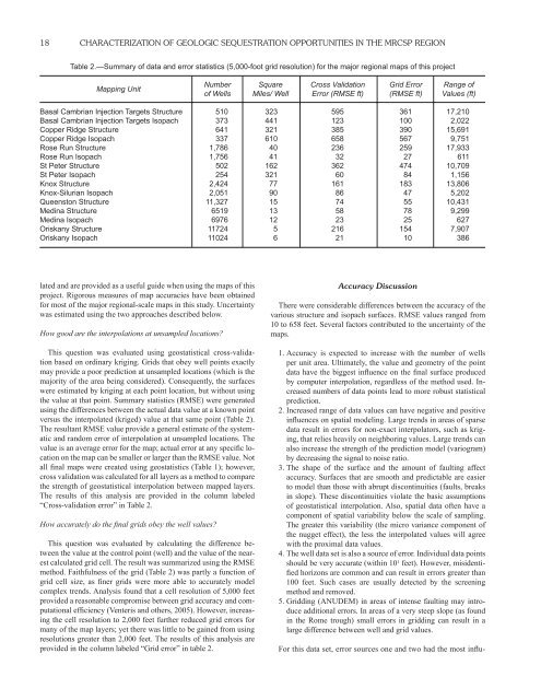
Table 2.—Summary of data and error statistics (5,000-foot grid resolution) for the major regional maps of this project
Mapping Unit
Number Square Cross Validation Grid Error Range of
of Wells Miles/ Well Error (RMSE ft) (RMSE ft) Values (ft)
Basal Cambrian Injection Targets Structure 510 323 595 361 17,210
Basal Cambrian Injection Targets Isopach 373 441 123 100 2,022
Copper Ridge Structure 641 321 385 390 15,691
Copper Ridge Isopach 337 610 658 567 9,751
Rose Run Structure 1,786 40 236 259 17,933
Rose Run Isopach 1,756 41 32 27 611
St Peter Structure 502 162 362 474 10,709
St Peter Isopach 254 321 60 84 1,156
Knox Structure 2,424 77 161 183 13,806
Knox-Silurian Isopach 2,051 90 86 47 5,202
Queenston Structure 11,327 15 74 55 10,431
Medina Structure 6519 13 58 78 9,299
Medina Isopach 6976 12 23 25 627
Oriskany Structure 11724 5 216 154 7,907
Oriskany Isopach 11024 6 21 10 386
lated and are provided as a useful guide when using the maps of this
project. Rigorous measures of map accuracies have been obtained
for most of the major regional-scale maps in this study. Uncertainty
was estimated using the two approaches described below.
How good are the interpolations at unsampled locations
This question was evaluated using geostatistical cross-validation
based on ordinary kriging. Grids that obey well points exactly
may provide a poor prediction at unsampled locations (which is the
majority of the area being considered). Consequently, the surfaces
were estimated by kriging at each point location, but without using
the value at that point. Summary statistics (RMSE) were generated
using the differences between the actual data value at a known point
versus the interpolated (kriged) value at that same point (Table 2).
The resultant RMSE value provide a general estimate of the systematic
and random error of interpolation at unsampled locations. The
value is an average error for the map; actual error at any specific location
on the map can be smaller or larger than the RMSE value. Not
all final maps were created using geostatistics (Table 1); however,
cross validation was calculated for all layers as a method to compare
the strength of geostatistical interpolation between mapped layers.
The results of this analysis are provided in the column labeled
“Cross-validation error” in Table 2.
How accurately do the fi nal grids obey the well values
This question was evaluated by calculating the difference between
the value at the control point (well) and the value of the nearest
calculated grid cell. The result was summarized using the RMSE
method. Faithfulness of the grid (Table 2) was partly a function of
grid cell size, as finer grids were more able to accurately model
complex trends. Analysis found that a cell resolution of 5,000 feet
provided a reasonable compromise between grid accuracy and computational
efficiency (Venteris and others, 2005). However, increasing
the cell resolution to 2,000 feet further reduced grid errors for
many of the map layers; yet there was little to be gained from using
resolutions greater than 2,000 feet. The results of this analysis are
provided in the column labeled “Grid error” in table 2.
Accuracy Discussion
There were considerable differences between the accuracy of the
various structure and isopach surfaces. RMSE values ranged from
10 to 658 feet. Several factors contributed to the uncertainty of the
maps.
1. Accuracy is expected to increase with the number of wells
per unit area. Ultimately, the value and geometry of the point
data have the biggest influence on the final surface produced
by computer interpolation, regardless of the method used. Increased
numbers of data points lead to more robust statistical
prediction.
2. Increased range of data values can have negative and positive
influences on spatial modeling. Large trends in areas of sparse
data result in errors for non-exact interpolators, such as kriging,
that relies heavily on neighboring values. Large trends can
also increase the strength of the prediction model (variogram)
by decreasing the signal to noise ratio.
3. The shape of the surface and the amount of faulting affect
accuracy. Surfaces that are smooth and predictable are easier
to model than those with abrupt discontinuities (faults, breaks
in slope). These discontinuities violate the basic assumptions
of geostatistical interpolation. Also, spatial data often have a
component of spatial variability below the scale of sampling.
The greater this variability (the micro variance component of
the nugget effect), the less the interpolated values will agree
with the proximal data values.
4. The well data set is also a source of error. Individual data points
should be very accurate (within 10 1 feet). However, misidentified
horizons are common and can result in errors greater than
100 feet. Such cases are usually detected by the screening
method and removed.
5. Gridding (ANUDEM) in areas of intense faulting may introduce
additional errors. In areas of a very steep slope (as found
in the Rome trough) small errors in gridding can result in a
large difference between well and grid values.
For this data set, error sources one and two had the most influ-