MRCSP Phase I Geologic Characterization Report - Midwest ...

More documents

Recommendations

Info

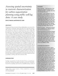
22 CHARACTERIZATION OF GEOLOGIC SEQUESTRATION OPPORTUNITIES IN THE MRCSP REGION industrial-waste injection well, 2) Class II—brine injection well, and 3) Class III—solution mining well. Locating all of these wells had never been accomplished before by all of the MRCSP project members; this information is usually kept by state or federal regulatory agencies. However, information about these wells, especially the Class I and II wells (Figure 13) will be crucial in understanding the injection characteristics of many of the target formations under consideration. Therefore, under Phase II of the MRCSP Partnership, the geologic team will obtain as much information as possible from these injection operations. Salinity Grid A salinity grid can be generated from mapping, either by direct interpolation (Kriging etc.) or by exploiting the general relationship of salinity increasing with depth. Mapping salinity accurately in this region is difficult because the data needed are not routinely gathered and submitted to state agencies; therefore the coverage is sparse. For example, the Mount Simon Sandstone has only 18 measurements of salinity scattered across the MRCSP area. In addition, formation waters are continuously modified by filtration through clay membranes, ion exchange reactions, precipitation of minerals, and by the solutioning of the surrounding rocks (Blatt and others, 1980), causing further uncertainty. For these reasons, a statistical salinity verses depth model was used to create the salinity grids used in capacity calculations for this investigation. The model was constructed from existing sample data using least-squares regression. Individual models were created for each formation and used with the overburden (depth) maps to make a continuous salinity grid for each formation. Geothermal Gradient and Temperature Models of the surface temperature and geothermal gradient were created to calculate the temperature at depth for use in the capacity calculations. For the surface temperature, the thirty-year average for over 275 cities was obtained for the conterminous United States (NOAA, 2000). The temperatures were interpolated into a grid using a minimum curvature algorithm. For the geothermal gradient, a number of datasets were investigated. These datasets included the American Association of Petroleum Geologists (AAPG) bottom-hole temperature dataset (AAPG, 1994), the Southern Methodist University (SMU) dataset (Blackwell and Richards, 2004a), and the 2004 AAPG heat flow dataset (Blackwell and Richards, 2004b). Each dataset was evaluated for data quality and spatial distribution. The AAPG heat flow dataset (Blackwell and Richards, 2004b) was not used because the data distribution was considered too sparse in the project area—only three heat flow measurements were for Ohio. The 1994 AAPG geothermal dataset was unsatisfactory because it was uncorrected for thermal equilibrium and, when analyzed using spatial statistics, the spatial variance was quite large. Of those evaluated, the SMU dataset (Blackwell and Richards, 2004a) was the best for this project because it combined a good combination of data coverage and quality. A regional correction was applied, which significantly reduced the spatial variance. In areas where the SMU dataset was missing data, such as Pennsylvania, data from the AAPG bottom hole temperature dataset (AAPG, 1994) was used to augment the SMU dataset. The augmented SMU dataset was used to create the geothermal gradient grid for the region using kriging in Geostatistical Analyst. Screening Maps The large number of maps, data grids, and calculations generated in this regional assessment make it difficult for the public, or any other user, to interpret the various attributes related to CO 2 sequestration in geologic units in the MRCSP study area.. Therefore, the geologic team has devising several methods to condense the various types of information contained herein into a smaller number of summary maps for quick reference, by both technical and non-technical audiences. Several techniques for creating summary maps were investigated. Approaches ranging from complex expert systems models, which codify qualitative geological knowledge numerical algorithms, to simple screening maps. Because the expert systems models rely on so much soft information (knowledge rather than data), it was decided, at this stage in the project, that simple Boolean screening maps were the best approach to presenting meaningful summaries. Quantifying geologic knowledge through expert systems approaches must be done with care and can be time consuming if realistic algorithms are to be developed. Research into more advanced techniques will continue in Phase II. A screening/planning map was produced using grids for all deep saline formations. Structure and isopach grids were reclassified into binary grids showing where the geology was appropriate and inappropriate for CO 2 injection, then reclassified to show areas where overburden thickness was greater than 3,000 feet (using the 2,500- foot rule of thumb for miscible injection, with 500 feet added to account for potential map error). Isopach grids were reclassified to show thicknesses greater than 50 feet. The reclassified grids were recombined into a single grid showing the number of appropriate targets and the name of the targets (Figure 14). This map can also be viewed as a 3-dimensional scene (Figure 15). The map is presented herein and will be discussed further with various stakeholder groups, including the partnership sponsors, to elicit input on its usefulness, clarity, and how it can be improved and added-to for development in Phase II. DATA STORAGE AND DISTRIBUTION Geologic data for this project is provided in both digital and as hard copy (paper) map formats. This was done to ensure that the needs of a wide range of stakeholders were met. The approach allows information to be distributed to individuals ranging from sophisticated GIS modelers to non-technical users who just need a map for a planning meeting. Data Storage All GIS data is being stored in a centralized ArcSDE database maintained by the Ohio Division of Geological Survey. For geologic target and confining layers, there are contour and grid data, geologic unit crop lines, and fault locations stored. Point data used in mapping are stored as a database containing all formation tops with a listing of basic well-header data (i.e., well operator, location, producing formation, well status, etc.). The database also contains all GIS layers created in this project, including layers from the terrestrial studies, CO 2 sources, surface digital-elevation model, oil and gas fields, and the various data and grids needed for capacity calculations. The database may be queried to obtain data for an individual geologic layer, by formation, depth, location, or any combination the user requires.
GEOLOGIC MAPPING PROCEDURES, DATA SOURCES AND METHODOLOGY 23 EXPLANATION Injection Wells Class I Class II P R O J E C T L I M I T 50 25 0 50 100 Miles 50 25 0 50 100 150 Kilometers ³ Figure 13.—Locations of Class I (hazardous and industrial waste) and Class II (oil field brine) injection wells.
Page 1 and 2: Characterization of Geologic Seques
Page 3 and 4: ABOUT THE MRCSP The Midwest Regiona
Page 5 and 6: CONTENTS About the MRCSP ..........
Page 7 and 8: CONTENTS Figure A14-2.—Structure
Page 9 and 10: 1 CHARACTERIZATION OF GEOLOGIC SEQU
Page 11 and 12: BACKGROUND INFORMATION 3 (a minimum
Page 13 and 14: INTRODUCTION TO THE MRCSP REGION’
Page 21 and 22: GEOLOGIC MAPPING PROCEDURES, DATA S
Page 29: GEOLOGIC MAPPING PROCEDURES, DATA S
Page 35 and 36: OIL, GAS, AND GAS STORAGE FIELDS 27
Page 41 and 42: CO 2-SEQUESTRATION STORAGE CAPACITY
Page 53 and 54: CONCLUSIONS AND REGIONAL ASSESSMENT
Page 55 and 56: REFERENCES CITED 47 National Confer
Page 57 and 58: 49 APPENDIX A Geologic Summaries of
Page 59 and 60: APPENDIX A: PRECAMBRIAN UNCONFORMIT
Page 61 and 62: APPENDIX A: CAMBRIAN BASAL SANDSTON
Page 67 and 68: APPENDIX A: BASAL SANDSTONES TO TOP
Page 73 and 74: APPENDIX A: UPPER CAMBRIAN ROSE RUN
Page 81 and 82:
APPENDIX A: KNOX TO LOWER SILURIAN
Page 83 and 84:
Page 85 and 86:
Page 87 and 88:
N T R APPENDIX A: KNOX TO LOWER SIL
Page 89 and 90:
APPENDIX A: MIDDLE ORDOVICIAN ST. P
Page 91 and 92:
-6000 -8000 APPENDIX A: MIDDLE ORDO
Page 93 and 94:
APPENDIX A: LOWER SILURIAN MEDINA G
Page 95 and 96:
Page 97 and 98:
Page 99 and 100:
Page 101 and 102:
APPENDIX A: NIAGARAN/LOCKPORT THROU
Page 103 and 104:
APPENDIX A: NIAGARAN/LOCKPORT THROU
Page 105 and 106:
A APPENDIX A: NIAGARAN/LOCKPORT THR
Page 107 and 108:
APPENDIX A: MIDDLE SILURIAN NIAGARA
Page 109 and 110:
-3000 APPENDIX A: MIDDLE SILURIAN N
Page 111 and 112:
APPENDIX A: LOWER DEVONIAN MANDATA
Page 113 and 114:
APPENDIX A: LOWER DEVONIAN ORISKANY
Page 115 and 116:
Page 117 and 118:
Page 119 and 120:
Page 121 and 122:
APPENDIX A: LOWER DEVONIAN SYLVANIA
Page 123 and 124:
-2000 APPENDIX A: LOWER DEVONIAN SY
Page 125 and 126:
25 APPENDIX A: LOWER/MIDDLE DEVONIA
Page 127 and 128:
APPENDIX A: DEVONIAN ORGANIC-RICH S
Page 129 and 130:
Page 131 and 132:
Page 133 and 134:
Page 135 and 136:
( ( ( ( APPENDIX A: PENNSYLVANIAN C
Page 137 and 138:
APPENDIX A: PENNSYLVANIAN COAL BEDS
Page 139 and 140:
Page 141 and 142:
Page 143 and 144:
APPENDIX A: LOWER CRETACEOUS WASTE
Page 145 and 146:
Page 147 and 148:
Page 149 and 150:
Page 151 and 152:
APPENDIX A: REFERENCES CITED 143 Sa
Page 153 and 154:
APPENDIX A: REFERENCES CITED 145 an
Page 155 and 156:
APPENDIX A: REFERENCES CITED 147 lo
Page 157 and 158:
APPENDIX A: REFERENCES CITED 149 Pa
Page 159 and 160:
APPENDIX A: REFERENCES CITED 151 Th
show all

MRCSP Phase I Geologic Characterization Report - Midwest ...

You also want an ePaper? Increase the reach of your titles

Delete template?

Save as template?