Physical Principles of Electron Microscopy: An Introduction to TEM ...
Physical Principles of Electron Microscopy: An Introduction to TEM ...
Physical Principles of Electron Microscopy: An Introduction to TEM ...

Create successful ePaper yourself
Turn your PDF publications into a flip-book with our unique Google optimized e-Paper software.
126 Chapter 5<br />
specimen<br />
scan<br />
coils<br />
objective<br />
lens<br />
z<br />
x<br />
specimen<br />
electron gun<br />
condenser<br />
lenses<br />
detec<strong>to</strong>r<br />
x<br />
y<br />
magnification<br />
control<br />
scan<br />
genera<strong>to</strong>rs<br />
signal<br />
amplifier<br />
display<br />
device<br />
image<br />
scan<br />
Figure 5-1. Schematic diagram <strong>of</strong> a scanning electron microscope with a CRT display.<br />
Above the specimen, there are typically two or three lenses, which act<br />
somewhat like the condenser lenses <strong>of</strong> a <strong>TEM</strong>. But whereas the <strong>TEM</strong>, if<br />
operating in imaging mode, has a beam <strong>of</strong> diameter � 1 �m or more at the<br />
specimen, the incident beam in the SEM (also known as the electron probe)<br />
needs <strong>to</strong> be as small as possible: a diameter <strong>of</strong> 10 nm is typical and 1 nm is<br />
possible with a field-emission source. The final lens that forms this very<br />
small probe is named the objective; its performance (including aberrations)<br />
largely determines the spatial resolution <strong>of</strong> the instrument, as does the<br />
objective <strong>of</strong> a <strong>TEM</strong> or a light-optical microscope. In fact, the resolution <strong>of</strong> an<br />
SEM can never be better than its incident-probe diameter, as a consequence<br />
<strong>of</strong> the method used <strong>to</strong> obtain the image.<br />
Whereas the conventional <strong>TEM</strong> uses a stationary incident beam, the<br />
electron probe <strong>of</strong> an SEM is scanned horizontally across the specimen in two<br />
perpendicular (x and y) directions. The x-scan is relatively fast and is<br />
generated by a saw<strong>to</strong>oth-wave genera<strong>to</strong>r operating at a line frequency fx ; see<br />
Fig. 5-2a. This genera<strong>to</strong>r supplies scanning current <strong>to</strong> two coils, connected in<br />
series and located on either side <strong>of</strong> the optic axis, just above the objective<br />
lens. The coils generate a magnetic field in the y-direction, creating a force<br />
on an electron (traveling in the z-direction) that deflects it in the x-direction;<br />
see Fig. 5-1.<br />
The y-scan is much slower (Fig. 5-2b) and is generated by a second<br />
saw<strong>to</strong>oth-wave genera<strong>to</strong>r running at a frame frequency fy = fx /n where n is<br />
an integer. The entire procedure is known as raster scanning and causes the<br />
beam <strong>to</strong> sequentially cover a rectangular area on the specimen (Fig. 5-2d).