Physical Principles of Electron Microscopy: An Introduction to TEM ...

36 Chapter 2
cross-product or vector product of v and B ; this mathematical operator
gives
Eq. (2.4) the following two properties.
1. The direction of F is perpendicular to both v and B. Consequently, F has
no component in the direction of motion, implying that the electron speed v
(the magnitude of the velocity v) remains constant at all times. But because
the direction of B (and possibly v) changes continuously, so does the
direction
of the magnetic force.
2. The magnitude F of the force is given by:
F = e v B sin(�) (2.5)
where � is the instantaneous angle between v and B at the location of the
electron. Because B (and possibly v) changes continuously as an electron
passes through the field, so does F. Note that for an electron traveling along
the coil axis, v and B are always in the axial direction, giving � = 0 and F = 0
at every point, implying no deviation of the ray path from a straight line.
Therefore,
the symmetry axis of the magnetic field is the optic axis.
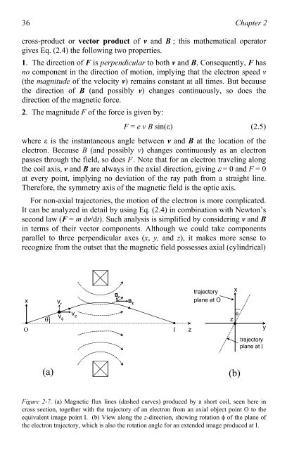
For non-axial trajectories, the motion of the electron is more complicated.
It can be analyzed in detail by using Eq. (2.4) in combination with Newton’s
second law (F = m dv/dt). Such analysis is simplified by considering v and B
in terms of their vector components. Although we could take components
parallel to three perpendicular axes (x, y, and z), it makes more sense to
recognize from the outset that the magnetic field possesses axial (cylindrical)
x
vr Br Bz trajectory
plane at O
v� vz �
z
�
O I z
(a) (b)
x
y
trajectory
plane at I
Figure 2-7. (a) Magnetic flux lines (dashed curves) produced by a short coil, seen here in
cross section, together with the trajectory of an electron from an axial object point O to the
equivalent image point I. (b) View along the z-direction, showing rotation � of the plane of
the electron trajectory, which is also the rotation angle for an extended image produced at I.