- Page 2 and 3:
Practical Data Acquisition forInstr
- Page 4 and 5:
Practical Data Acquisition forInstr
- Page 6 and 7:
In less than a decade, the PC has b
- Page 8 and 9:
PrefaceContentsxvii1 Introduction 1
- Page 10 and 11:
Contents vii4.2.1 Hardware interrup
- Page 12 and 13:
Contents ix6.2.3 Functional descrip
- Page 14 and 15:
Contents xi9.1 Ethernet and fieldbu
- Page 16 and 17:
Contents xiii12.5.2 Pin assignments
- Page 18 and 19:
Contents xvType R thermocouple 384T
- Page 20 and 21:
A data acquisition and control syst
- Page 22 and 23:
FilteringIn noisy environments, it
- Page 24 and 25:
are capable of programmed I/O and i
- Page 26 and 27:
Plug-in expansion boards are common
- Page 28 and 29:
50 mRS-232 Communication InterfaceS
- Page 30 and 31:
speeds are of the order of 1 Mbyte/
- Page 32 and 33:
14 Practical Data Acquisition for I
- Page 34 and 35:
16 Practical Data Acquisition for I
- Page 36 and 37:
18 Practical Data Acquisition for I
- Page 38 and 39:
20 Practical Data Acquisition for I
- Page 40 and 41:
22 Practical Data Acquisition for I
- Page 42 and 43:
24 Practical Data Acquisition for I
- Page 44 and 45:
26 Practical Data Acquisition for I
- Page 46 and 47:
28 Practical Data Acquisition for I
- Page 48 and 49:
30 Practical Data Acquisition for I
- Page 50 and 51:
32 Practical Data Acquisition for I
- Page 52 and 53:
34 Practical Data Acquisition for I
- Page 54 and 55:
3PC based data acquisition (DAQ) sy
- Page 56 and 57:
3.2.3 FilteringIsolation performs s
- Page 58 and 59:
The transfer characteristics of a p
- Page 60 and 61:
Figure 3.7Ideal band pass filter tr
- Page 62 and 63:
Figure 3.11Two-stage Butterworth fi
- Page 64 and 65:
As individual signal conditioning m
- Page 66 and 67:
ThermocouplesDigitalTransmitterDigi
- Page 68 and 69:
Examples of floating signal sources
- Page 70 and 71:
espect to the measurement system gr
- Page 72 and 73:
Figure 3.26Opto-coupler isolation o
- Page 74 and 75:
• Using isolation amplifiers to i
- Page 76 and 77:
Figure 3.31Physical representation
- Page 78 and 79:
field or if the field is caused by
- Page 80 and 81:
Where the shield is grounded (i.e.
- Page 82 and 83:
mines the amount of noise in the ci
- Page 84 and 85:
For full-duplex systems using balan
- Page 86 and 87:
4.1.1 DOSusually consist of a small
- Page 88 and 89:
With the advent of Windows as a gra
- Page 90 and 91:
UNIX shellSimilar to the DOS comman
- Page 92 and 93:
available to the expansion bus. A l
- Page 94 and 95:
4.2.7 Interrupt service routinesIt
- Page 96 and 97:
Whichever CPU is being used, it mus
- Page 98 and 99:
• An I/O device requests a DMA tr
- Page 100 and 101:
Normal DMA using on-board FIFOThe D
- Page 102 and 103:
ferring samples until the counter r
- Page 104 and 105:
The read or write command signals (
- Page 106 and 107:
Shortened 3-BCLK 8-bit memory acces
- Page 108 and 109:
Extended 6-BCLK 16-bit memory acces
- Page 110 and 111:
• A cycle which the expansion boa
- Page 112 and 113:
Figure 4.13Timing chart of a shorte
- Page 114 and 115:
Figure 4.15Timing chart of an exten
- Page 116 and 117:
4.7.2 Expanded memory system (EMS)E
- Page 118 and 119:
The IBM PC and early versions of th
- Page 120 and 121:
Figure 4.17ISA signal mnemonics, si
- Page 122 and 123:
data bus. An example of this happen
- Page 124 and 125:
NOWSThe /NOWS (NO wait state) signa
- Page 126 and 127:
interrupt lines (1RQ13, 8, 2, 1 and
- Page 128 and 129:
one application at a time, it is ne
- Page 130 and 131:
The need for PCs to exchange data w
- Page 132 and 133:
Figure 4.198-bit 21-line I/O board4
- Page 134 and 135:
Address decoding on the 24-line pro
- Page 136 and 137:
The write cycle is considered in th
- Page 138 and 139:
data acquisition and control system
- Page 140 and 141:
Adjustable on-board fixed gain ampl
- Page 142 and 143:
level applied at the input. When a
- Page 144 and 145:
Each step effectively divides the r
- Page 146 and 147:
The operation of a dual slope integ
- Page 148 and 149:
Code widthThis is the fundamental q
- Page 150 and 151:
(a) Unipolar offset error(b) Bipola
- Page 152 and 153:
Changes in temperature result in a
- Page 154 and 155:
1 LSB. Therefore, an ideal A/D conv
- Page 156 and 157:
• The source and level of interru
- Page 158 and 159:
5.3.3 Differential inputsTrue diffe
- Page 160 and 161:
A/D board can divide the input rang
- Page 162 and 163:
a) DC alias caused by sampling at h
- Page 164 and 165:
Figure 5.15Frequency spectrum of or
- Page 166 and 167:
ate be a minimum of about five time
- Page 168 and 169:
Figure 5.20Many aliases combined wi
- Page 170 and 171:
initiated. The data is subsequently
- Page 172 and 173:
Figure 5.22Time skew between channe
- Page 174 and 175:
For each burst trigger, the A/D boa
- Page 176 and 177:
Analog output D/A boardsUnlike high
- Page 178 and 179:
Like the weighted-current source ne
- Page 180 and 181:
The generation of high frequency si
- Page 182 and 183:
• The plug-in connector, which pr
- Page 184 and 185:
Latched digital I/OFor applications
- Page 186 and 187:
y increasing the resistance of R x
- Page 188 and 189:
One advantage of this type of relay
- Page 190 and 191:
Figure 5.36Waveforms showing genera
- Page 192 and 193:
When a counter is configured to ena
- Page 194 and 195:
6The standardization of the RS-232
- Page 196 and 197:
A duplex system is designed for sen
- Page 198 and 199:
Some examples of the HEX and BIN va
- Page 200 and 201:
In summary, the optional settings f
- Page 202 and 203:
At the RS-232 receiver the followin
- Page 204 and 205:
110 850300 800600 7001200 5002400 2
- Page 206 and 207:
• Pin 7: Signal ground (common)Th
- Page 208 and 209:
6.2.5 Examples of RS-232 interfaces
- Page 210 and 211:
terminating resistors, approximatel
- Page 212 and 213:
Another commonly used technique, ba
- Page 214 and 215:
• Line controlThis applies to hal
- Page 216 and 217:
The calculation of the block checks
- Page 218 and 219:
The mechanism of operation of the C
- Page 220 and 221:
Figure 6.18, has appropriate intern
- Page 222 and 223:
77.1 IntroductionAs with other form
- Page 224 and 225:
inserted in the device. This is its
- Page 226 and 227:
How frequently logged data is uploa
- Page 228 and 229:
The following hardware components d
- Page 230 and 231:
In a typical stand-alone data acqui
- Page 232 and 233:
The maximum battery life that can b
- Page 234 and 235:
Input termination resistors, typica
- Page 236 and 237:
Figure 7.13 shows the standard conn
- Page 238 and 239:
interface, even at high speed, the
- Page 240 and 241:
• Use different data formats so t
- Page 242 and 243:
Command errors are reported immedia
- Page 244 and 245:
• Channel scalingThis automatical
- Page 246 and 247:
The channel scan for this type of s
- Page 248 and 249:
Data is logged in a fixed non-ASCII
- Page 250 and 251:
7.9 Stand-alone logger/controllers
- Page 252 and 253:
88.1 IntroductionThe communications
- Page 254 and 255: Figure 8.2GPIB connector (IEEE 488)
- Page 256 and 257: • TalkersA talker is a one-way co
- Page 258 and 259: controller in charge (CIC). The IFC
- Page 260 and 261: Each device connected to the GPIB h
- Page 262 and 263: One of the additional features that
- Page 264 and 265: • The controller temporarily conf
- Page 266 and 267: Table 8.4IEEE 488.2 commandsThe SCP
- Page 268 and 269: Figure 8.9SCPI instrument modelThe
- Page 270 and 271: 99.1 Ethernet and fieldbuses for da
- Page 272 and 273: cabling tray etc and the transceive
- Page 274 and 275: transceiver in the MAU and this is
- Page 276 and 277: Advantages of the system include:
- Page 278 and 279: of a cell as well, but these are ig
- Page 280 and 281: Figure 9.8CSMA/CD collisionsAssume
- Page 282 and 283: • PreambleThis field consists of
- Page 284 and 285: of this figure. Some manufacturers
- Page 286 and 287: Grounding has safety and noise conn
- Page 288 and 289: Just as with any technology, each o
- Page 290 and 291: information. The packet is then pla
- Page 292 and 293: There are two types of connectors,
- Page 294 and 295: HOSTClient SoftwareManages Interfac
- Page 296 and 297: Figure 10.6USB connector pinsThere
- Page 298 and 299: The idle states for low- and high-s
- Page 300 and 301: The interrupt transfer type is used
- Page 302 and 303: than in spending a lot of time and
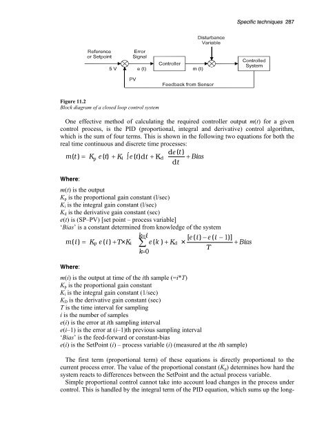
- Page 306 and 307: term error (m) in the system and ad
- Page 308 and 309: 11.2 Capturing high speed transient
- Page 310 and 311: 12IntroductionThe PCMCIA (PCMCIA st
- Page 312 and 313: adapter on a full size computer has
- Page 314 and 315: Pager cards are used in offices and
- Page 316 and 317: Size 85.6 mm × 54.0 mmType I 3.3 m
- Page 318 and 319: The memory only interface is conver
- Page 320 and 321: The AIMS interface supports large d
- Page 322 and 323: 12.8 FutureThe card information str
- Page 324 and 325: A/D conversion timeAddressAddress r
- Page 326 and 327: Back-planeBand pass filterBandwidth
- Page 328 and 329: BufferBusBWCache memoryCCDCCIRCCITT
- Page 330 and 331: pixel is subjected to a mathematica
- Page 332 and 333: data between the computer memory an
- Page 334 and 335: FrameFrame grabberFringingFull dupl
- Page 336 and 337: so that they interlock. The PAL sta
- Page 338 and 339: Lux-secondSI unit of light exposure
- Page 340 and 341: NTSCNull modemNumber of channelsNyq
- Page 342 and 343: PortPPIPre-triggerProgram I/OProgra
- Page 344 and 345: whereby the first gray level of eac
- Page 346 and 347: allowing the user to control basic
- Page 348 and 349: input.TrunkUARTUnipolar inputsUnloa
- Page 350 and 351: Appendix BThe information in this s
- Page 352 and 353: Table B.4Controller 2: 16-bit (AT o
- Page 354 and 355:
B.5 8253/8254 Counter/timer
- Page 356:
Table B.8Memory map for PC/XT/AT
- Page 359 and 360:
Table B.10BIOS data area
- Page 361 and 362:
Table B.15ROMTable B.16AT extended
- Page 363 and 364:
← ↔ ← ← ← ↔
- Page 365 and 366:
Figure B.1Card dimensions for PC/XT
- Page 367 and 368:
Appendix CThis section contains bri
- Page 369 and 370:
the control register of the 8255. T
- Page 371 and 372:
The bits A7 (MSB) down to A0 (LSB)
- Page 373 and 374:
Table C.6Instructions for reading o
- Page 375 and 376:
The program could also enable the I
- Page 377 and 378:
Group AConfiguration Informationto
- Page 379 and 380:
C.11 Single-bit set/resetAny of the
- Page 381 and 382:
Figure C.15Bi-directional bus (mode
- Page 383 and 384:
Figure D.18254 Block diagramFigure
- Page 385 and 386:
Figure D.3TCCTRL registerThe functi
- Page 387 and 388:
This is the data register of the fi
- Page 389 and 390:
• A simple read operation• A co
- Page 391 and 392:
The null count bit indicates if the
- Page 393 and 394:
For even counts: the output is init
- Page 395 and 396:
Appendix EThe IPTS-68 standard defi
- Page 397 and 398:
Number of ranges = 2Range #1 -270 t
- Page 399 and 400:
Number of ranges = 1Range #1 -210 t
- Page 401 and 402:
Range #2 0 to 1372°COrder of polyn
- Page 403 and 404:
Number of Ranges = 4Range #1 -50 to
- Page 405 and 406:
Number of ranges = 2Range #1 -270 t
- Page 407 and 408:
Appendix FF.1 IntroductionAll activ
- Page 409 and 410:
Table F.3 gives the conversion betw
- Page 411 and 412:
The conversion between binary and h
- Page 413 and 414:
F.8 Internal representation of info
- Page 415 and 416:
12 which is equivalent to: 1100-4 S
- Page 417 and 418:
DCDCASDCISDCLDDDIODTDTASDTISENDEOIE
- Page 419 and 420:
STBSTRSSWNST(T)TETACSTADSTAGTCATCST
- Page 421 and 422:
404 IndexDuplex:full duplex 178half
- Page 423 and 424:
406 IndexOpen loop control 285see a
- Page 425:
THIS BOOK WAS DEVELOPED BY IDC TECH