Edition

IFTA JOURNAL
2017 EDITION
The F-ratio is used to decide whether the overall model has
statistically significant predictive capability. To determine
the significance of the F-ratio, we can look at its associated
p-value. 8 In this paper, we will look for p-values smaller than
0.01. If the F-ratio calculated by mvreg is significant, we can
infer that the overall model has predictive capability.
After deciding which overall models have attractive measures
of goodness of fit, we “drill” down into the model to look at
the regression coefficient and t-statistic of each independent
variable to determine why.
The regression coefficient is a factor that determines how
each independent variable affects the dependent variable. For
example, if the past return has a negative regression coefficient,
the past return is modeled to decrease the prediction of the
future return (mean reversion). In the opposite case, if the past
return has a positive regression coefficient, the past return is
modeled to increase the prediction of the future return. The
regression coefficients are estimated parameters; therefore,
mvreg also calculates an associated error term. This error
term is called the Standard Error and is used to construct a
confidence interval for what the true regression coefficient
actually is.
The t-statistic is a ratio of the regression coefficient divided
by its Standard Error. Similar to the F-ratio, the t-statistic has
an associated p-value to help determine if it is significant or not.
Later, I will use these measures to examine two of the mvreg
output tables and reason through why one is a good predictor
model and why the other is a poor predictor model (Table 9 and
Table 10 in the 12-Month Look-Back Analysis section).
Optimal Time Period Analyses
3-Month Look Back Analysis
For a visualization of how the data is calculated, please refer
to Figure 1, substituting x = 3 for the independent variable
calculations and k = 3, 6, 12, 36 for the dependent variable
calculations.
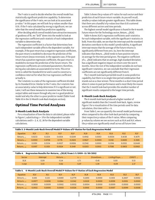
Table 3 shows the p-values of F-ratios for each sector and their
prediction of each future return variable. As you will recall,
smaller p-values indicate greater significance. This table shows
that there are a handful of p-values less than 0.01 scattered
across different sectors and time periods.
The highest overall model significance is found in the 6-month
future return for the Technology sector, Return t + 6 (XLK).
Table 4 shows XLK’s regression coefficients and t-statistics
for each independent variable, with the significant t-statistics in
bold. From this table, we see that the intercept and the standard
deviation contribute to this model’s predictability. A significant
intercept means that the average of the future returns is
significantly different from zero. So, here the intercept
indicates that Return t + 6 (XLK) tends to have positive returns
on average for the time period given. The negative coefficient
of s t − 3 (XLK) indicates that on average, high standard deviation
has a significant negative impact on return over the next 6
months. Since the rest of the independent variables do not have
significant t-statistics, we can conclude that their regression
coefficients are not significantly different from 0.
The 3-month look-back period did result in some predictive
capability, but there is no single time period combination that
stands out as a clear winner. Three months is a short time period
when it comes to past performance and is most likely the reason
that the 3-month look-back provides the smallest number of
significant results compared to the longer time periods.
6-Month Look-Back Analysis
The 6-month look-back produced a higher number of
significant models than the 3-month look-back. Again, review
Figure 1 for a visualization of the time periods used for data
calculation, this time with x = 6.
From Table 5, we can quantify the overall model performance
when compared to the other look-back periods by comparing
their respective p-values of the F-ratios. When comparing
p-values by column we see sectors such as XLK and XLF, where
the p-values are significantly small across all future time
Table 3. 3-Month Look-Back Overall Model P-Values of F-Ratios for Each Regression Model
Equation XLV XLI XLY XLP XLB XLK XLU XLE XLF
Return t + 3 0.0233 0.1254 0.6354 0.0249 0.4942 0.0053 0.0034 0.4138 0.1679
Return t + 6 0.0303 0.4758 0.776 0.2424 0.9627 0.0000 0.042 0.6683 0.3185
Return t + 12 0.0191 0.3134 0.0027 0.0056 0.2342 0.0001 0.1194 0.0315 0.0449
Return t + 36 0.0197 0.1301 0.0024 0.1149 0.0203 0.0015 0.7081 0.5803 0.0063
Table 4. Regression Results for Return t + 6(XLK) from 1/1/1999–11/30/2012
Sector Intercept Return t − 3 s t − 3 Drawdown t − 3 LinRegSlope t − 3 EXRET t − 3
XLK 0.09 -0.14 -1.71 -0.45 0.00 0.51
t-stat 3.53 -0.62 -5.07 -1.39 -0.09 2.17
Table 5.
6-Month Look-Back Overall Model P-Values for F-Ratios of Each Regression Model
Equation XLV XLI XLY XLP XLB XLK XLU XLE XLF
Return t + 3 0.001 0.125 0.6069 0.2779 0.2055 0.0000 0.1104 0.2607 0.0002
Return t + 6 0.0977 0.0208 0.1064 0.1542 0.0129 0.0000 0.0059 0.0051 0.0000
Return t + 12 0.0858 0.0009 0.0002 0.0032 0.0004 0.0000 0.0009 0.0000 0.0000
Return t + 36 0.0012 0.0000 0.0000 0.0326 0.0001 0.0000 0.0007 0.0099 0.0008
IFTA.ORG PAGE 111