Edition

IFTA JOURNAL
2017 EDITION
since Jegadeesh and Titman’s study depicts and reinforces the
profits of momentum over different facets in the markets.
Up to Antonacci (2012), momentum has been explored
from using either cross-sectional momentum or timeframe
momentum. In Antonacci’s Risk Premia Harvesting Through Dual
Momentum, he argues that using the two momentums in tandem
with each other will enhance the returns. The results generated
from the study portray exactly that, and further depict that
using them in tandem makes diversification more efficient.
Following Li, Xiaofei; Brooks, Chris; Miffre, Joelle (2009),
trading falling stocks is more “expensive” than trading booming
stocks. Through this idea, the paper “Low-Cost Momentum
Strategies” attempts to define a new momentum whereby there
is a relationship between the transaction costs and the volume
traded; this relationship only materializes when selling, not
when buying. The results reinforce the idea that “the strategies
that shortlist the 10%, 20% and 50% of winners and losers with
the lowest total transaction costs generate average net returns
of 18.24%, 15.84%, and 12.49%, respectively.” (page 12).
The Fama–French three-factor model was a method of
measuring market returns, and through research, it was
uncovered that value stocks outperform growth stocks. Carhart
(1997) provided an extension to the model and included another
factor—momentum; more specifically, monthly momentum, and
ultimately suggests that the four-factor model is predominantly
a more effective method of predicting market returns.
Methodology
Signaling
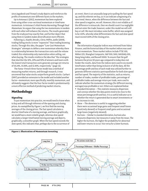
To put momentum into practice, we would need to know when
to buy and sell through inference of the opening and closing
prices. As exemplified by Figure 1, we first find the moving
averages of the closing prices. The fast speed calculates a
shorter timeframe of a moving average, and hence graphically,
we would have a more volatile graph, whereas slow speed
calculates a larger timeframed moving average and depicts,
graphically, a smoother graph. When the fast speed exceeds the
slow speed, this indicates that, perhaps due to the occurrence of
an event, there is an unusually large price pulling the fast speed
up, and this wherein we buy, as it can indicate a beginning of a
new trend. Hence, when the difference between the fast and
slow speed is negative, we sell. However, this is not reliable as if
the difference is minuscule, then we should count it as negligible
and not enter the trade; however, under this model we will still
buy or sell. We must introduce some buffer, which was assigned
to be 120%, whereby what differentiates the fast and slow speed
must exceed 120% of the closing price.
Data
The information of popular indices was retrieved from Yahoo
Finance, and the historical data of the market indices was used
to test momentum. These market indices include FTSE 100,
Nikkei 225, Shanghai Composite, S&P 500, DAX, NASDAQ-100,
Hang Seng Index, and Russell 3000. To ensure that the gulf
between the prices 50 years ago compared to today does not
hinder the results, data from the indices were used in six-month
timeframes rather than being inclusive of all the data. All the
percentage profit and loss of each trade was utilized further to
generate different statistics portrayed below for both slow speed
and fast speed. The majority of the statistics, such as returns,
number of trades, number of profitable trades, percentage of
profitable trades and average return per trade, were used to
indicate whether the momentum strategy (for different moving
averages) was profitable or not. Others are explained below:
• Standard Deviation – This statistic measures dispersion
and conveys whether the data points tend to be close to the
mean percentage profit and loss. It is a useful indicator as to
whether the return is generated due to smart investments or
an increase in risk.
• Skew – The skewness is useful in suggesting whether
there were occasional large gains and frequent small losses
(positively skewed) or frequent small gains and occasional
large losses (negatively skewed).
• Kurtosis – Similar to standard deviation, kurtosis also
measures dispersion, but measures it away from the mean. The
higher the kurtosis, the higher the probability for abnormal
and lower returns to occur. Vice versa for a lower kurtosis.
Figure 1. Illustration of Momentum Investing
PAGE 96
IFTA.ORG