Edition

IFTA JOURNAL
2017 EDITION
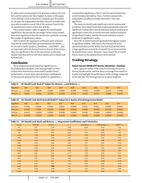
R 2 values were not presented in the previous analyses, but XLP,
XLY, and XLI achieve the three highest R 2 values in this paper,
so we will take a look at them here. Using the past 36 months
to calculate the independent variables resulted in models that
were able to explain around 50% of the variance found in the
36-month future return of XLP, XLY, and XLI.
The p-values found in Table 12 explain the overall model
significance. We see that the two longer future return models
have more significance than the shorter two, purely by counting
the number of significant p-values.
Table 13 shows the regression coefficients and t-statistics
from the 36-month look-back period prediction for Return t + 12 .
As we saw in earlier analyses, Drawdown t − x and EXRET t − x play
an important roll in the forward returns of most of the sectors.
They are significant in five of the nine sectors in the same
manner that they were in both the 6-month and 12-month look
back periods.
Conclusion
These analyses attached statistical significance to
five independent variables, over varying lengths of time,
to determine how history can be used to predict future
performance. In total, there were 16 unique combinations
of time periods analyzed for their predictive capabilities. I
evaluated the significance of the F-ratio for each to determine
overall model predictability. Then, I further evaluated the
independent variables of models where the F-ratio was
significant.
The count of overall model significance can be summarized
as follows: The 3-month look-back analysis produced a total of 9
significant F-ratios; the 6-month look-back analysis produced 23
significant F-ratios; the 12-month look-back analysis produced
29 significant F-ratios; and the 36-month look back analysis
produced 25 significant F-ratios.
Since the 12-month look-back generated the highest number
of significant models, I will choose this time period as the
optimal look-back period. Within this look-back period, there
is high significance in both the 12-month future return and the
36-month future return. However, I have chosen the 12-month
future return as the optimal future return period.
Trading Strategy
Select Sector SPDR ETF Sector Rotation—Outline
Here, I give an outline of the rules for selecting the sectors,
discuss the allocations and how they can change from month to
month, and highlight the performance of the strategy compared
to the S&P 500. This strategy will use an equal-weighted
Table 11. 36-Month Look-Back R 2 Values for Return t + 12 and Return t + 36
Equation XLV XLI XLY XLP XLB XLK XLU XLE XLF
Return t + 12 0.1284 0.2520 0.2987 0.2164 0.1892 0.1000 0.2039 0.3733 0.2786
Return t + 36 0.1605 0.4505 0.5402 0.5503 0.2118 0.1645 0.2711 0.2896 0.2337
Table 12.
36-Month Look-Back Overall Model P-Values for F-Ratios of Each Regression Model
Equation XLV XLI XLY XLP XLB XLK XLU XLE XLF
Return t + 3 0.0792 0.0645 0.0764 0.0524 0.0068 0.0135 0.2011 0.0002 0.0063
Return t + 6 0.7404 0.0155 0.0048 0.0096 0.0000 0.0818 0.0005 0.0000 0.0000
Return t + 12 0.0423 0.0000 0.0000 0.0000 0.0000 0.0196 0.0000 0.0000 0.0000
Return t + 36 0.0000 0.0000 0.0000 0.0000 0.0000 0.0004 0.0000 0.0000 0.0000
Table 13.
36-Month Look-Back and Return t + 12—Regression Coefficients and T-Statistics
Sector Intercept Return t − 36 s t − 36 Drawdown t − 36 LinRegSlope t − 36 EXRET t − 36
XLV 0.07 -0.07 -0.89 -0.60 0.00 0.22
t-stat 1.38 -0.3 -0.76 -2 1.96 1.7
XLI -0.17 0.88 3.05 -0.95 0.00 -1.01
t-stat -3.28 3.46 3.21 -3.33 -0.73 -3.47
XLY -0.16 -0.05 3.21 -0.68 0.00 0.28
t-stat -2.25 -0.21 2.26 -2.47 1.96 1.07
XLP -0.04 0.56 1.00 -1.47 0.00 -0.20
t-stat -1.03 2.27 0.79 -5.2 0.7 -1.71
XLB -0.09 0.46 2.40 -0.45 0.00 -0.64
t-stat -1.28 2.14 2.49 -1.76 -1.43 -3.6
XLK 0.06 0.02 -0.77 -0.59 0.00 0.31
t-stat 1.12 0.09 -0.86 -2.19 0.05 1.82
XLU -0.11 1.18 1.82 -1.34 0.00 -0.57
t-stat -1.72 4.6 1.35 -4.41 -0.86 -3.76
XLE 0.36 1.02 -4.01 -0.47 0.00 -0.95
t-stat 4.04 4.82 -3.1 -1.59 -5.71 -5.46
XLF -0.09 -0.68 1.07 -0.77 0.00 0.98
t-stat -1.66 -2.49 1.28 -2.57 4.38 4.14
PAGE 114
IFTA.ORG