Heiss W.D. (ed.) Quantum dots.. a doorway to - tiera.ru

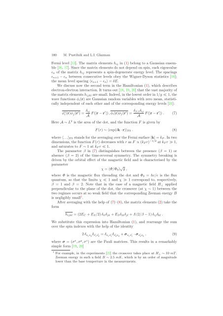
100 M. Pustilnik and L.I. Glazman
Fermi level [13]. The matrix elements hij in (1) belong to a Gaussian ensemble
[16, 17]. Since the matrix elements do not depend on spin, each eigenvalue
ɛn of the matrix hij represents a spin-degenerate energy level. The spacings
ɛn+1 − ɛn between consecutive levels obey the Wigner-Dyson statistics [16];
the mean level spacing 〈ɛn+1 − ɛn〉 = δE.
We discuss now the second term in the Hamiltonian (1), which describes
electron-electron interaction. It turns out [18, 19, 20] that the vast majority of
the matrix elements hijkl are small. Indeed, in the lowest order in 1/g ≪ 1, the
wave functions φi(r) are Gaussian random variables with zero mean, statistically
independent of each other and of the corresponding energy levels [21]:
φ ∗ i (r)φ j (r′ )= δij
A F (|r − r′ |) , φi(r)φj(r ′ )= δβ,1δij
A F (|r − r′ |) . (7)
Here A∼L 2 is the area of the dot, and the function F is given by
F (r) ∼〈exp(ik · r)〉FS . (8)
where 〈...〉FS stands for the averaging over the Fermi surface |k| = kF . In two
dimensions, the function F (r) decreases with r as F ∝ (kF r) −1/2 at kF r ≫ 1,
and saturates to F ∼ 1atkFr ≪ 1.
The parameter β in (7) distinguishes between the presence (β =1)or
absence (β = 2) of the time-reversal symmetry. The symmetry breaking is
driven by the orbital effect of the magnetic field and is characterised by the
parameter
χ =(Φ/Φ0) √ g,
where Φ is the magnetic flux threading the dot and Φ0 = hc/e is the flux
quantum, so that the limits χ ≪ 1andχ≫1 correspond to, respectively,
β = 1 and β = 2. Note that in the case of a magnetic field H⊥ applied
perpendicular to the plane of the dot, the crossover (at χ ∼ 1) between the
two regimes occurs at so weak field that the corresponding Zeeman energy B
is negligibly small1 .
After averaging with the help of (7)–(8), the matrix elements (2) take the
form
hijkl =(2EC + ES/2) δilδjk + ESδikδjl + Λ (2/β − 1) δijδkl .
We substitute this expression into Hamiltonian (1), and rearrange the sum
over the spin indexes with the help of the identity
2 δs 1 s 2 δs ′ 1 s′ 2 = δs 1 s ′ 1 δs ′ 2 s 2 + σs 1 s ′ 1 · σs ′ 2 s 2
, (9)
where σ =(σ x ,σ y ,σ z ) are the Pauli matrices. This results in a remarkably
simple form [19, 20]
1 For example, in the experiments [22] the crossover takes place at H⊥ ∼ 10 mT .
Zeeman energy in such a field B ∼ 2.5 mK, which is by an order of magnitude
lower than the base temperture in the measurements.