Heiss W.D. (ed.) Quantum dots.. a doorway to - tiera.ru

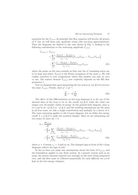
RG for Interacting Fermions 17
equations for the Vαβγδ. In principle this flow equation will involve all powers
of V but we will keep only quadratic terms (the one-loop approximation).
Then the diagrams are limited to the ones shown in Fig. 5, leading to the
following contributions to the scattering amplitude Γαβγδ
Γαβγδ = Vαβγδ
+ �
µ,ν
′ NF (ν) − NF (µ)
εµ − εν
− �
′ 1 − NF (µ) − NF (ν)
µν
εµ + εν
�
VανµδVβµνγ − VανµγVβµνδ
VαβµνVνµγδ
�
(31)
where the prime on the sum reminds us that only the g ′ remaining states are
to be kept and where NF (α) is the Fermi occupation of the state α. We will
confine ourselves to zero temperature where this number can only be zero
or one. The matrix element Vαβγδ now explicitly depends on the RG flow
parameter t.
Now we demand that upon integrating the two states at ±g ′ ∆/2 we recover
the same Γαβγδ. Clearly, since g ′ = ge −t ,
d δ
= −g′
dt δg ′
(32)
The effect of this differentiation on the loop diagrams is to fix one of the
internal lines of the loop to be at the cutoff ±g ′ ∆/2, while the other one
ranges over all smaller values of energy. In the particle-hole diagram, since µ
or ν can be at +g ′ ∆/2 or−g ′ ∆/2, and the resulting summations are the same
in all four cases, we take a single contribution and multiply by a factor of 4.
The same reasoning applies to the Cooper diagram. Let us define the energy
cutoff Λ = g ′ ∆/2 to make the notation simpler. Since we are integrating out
two states we have δg ′ =2
0= dVαβγδ
dt
− g′ �
′
4
2
µ=Λ,ν
NF (ν) − NF (µ)
εµ − εν
+ g′ �
4
2 εµ + εν
µ=Λ,ν
�
′ 1 − NF (µ) − NF (ν)
VανµδVβµνγ − VανµγVβµνδ
VαβµνVνµγδ
�
(33)
where µ = Λ means εµ = Λ and so on. The changed sign in front of the 1-loop
diagrams reflects the sign of (32)
So far we have not made any assumptions about the form of Vαβγδ, and
the formulation applies to any finite system. In a generic system such as an
atom, the matrix elements depend very strongly on the state being integrated
over, and the flow must be followed numerically for each different set αβγδ
kept in the low-energy subspace.