Heiss W.D. (ed.) Quantum dots.. a doorway to - tiera.ru

8 R. Shankar
the outgoing ones are forced to be equal to them (not in their sum, but
individually) up to a permutation, which is irrelevant for spinless fermions.
Thus we have in the end just one function of two angles, and by rotational
invariance, their difference:
u(θ1,θ2,θ1,θ2) =F (θ1 − θ2) ≡ F (θ) . (16)
About forty years ago Landau came to the very same conclusion [3] thata
Fermi system at low energies would be described by one function defined on
the Fermi surface. He did this without the benefit of the RG and for that
reason, some of the leaps were hard to understand. Later detailed diagrammatic
calculations justified this picture [4]. The RG provides yet another way
to understand it. It also tells us other things, as we will now see.
The first thing is that the final angles are not slaved to the initial ones if
the former are exactly opposite, as in the right half of Fig. 2. In this case, the
final ones can be anything, as long as they are opposite to each other. This
leads to one more set of marginal couplings in the BCS channel, called
u(θ1, −θ1,θ3, −θ3) =V (θ3 − θ1) ≡ V (θ) . (17)
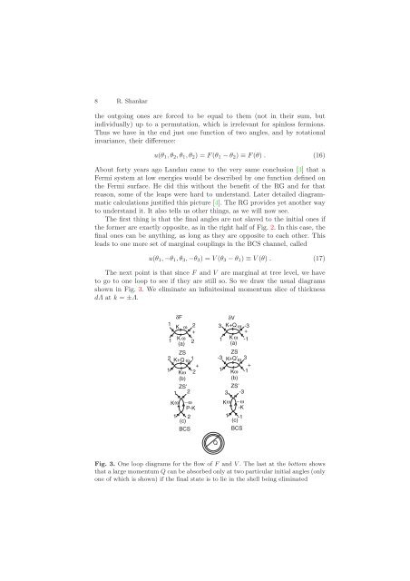
The next point is that since F and V are marginal at tree level, we have
to go to one loop to see if they are still so. So we draw the usual diagrams
showninFig.3. We eliminate an infinitesimal momentum slice of thickness
dΛ at k = ±Λ.
δF δV
1
K ω 2
+
3 K+Q ω -3
+
1
K ω
(a)
2 1 K ω
(a)
-1
ZS
2 K +Q ω 1
+
1
K ω 2
(b)
ZS’
1 2
K ω
− ω
P-K
1 2
(c)
BCS
Q
ZS
-3 K +Q’ ω 3
+
1
K ω -1
(b)
ZS’
3 -3
K ω
− ω
-K
1 -1
(c)
BCS
Fig. 3. One loop diagrams for the flow of F and V . The last at the bottom shows
that a large momentum Q can be absorbed only at two particular initial angles (only
one of which is shown) if the final state is to lie in the shell being eliminated