download completo - SET - USP

A mixed BEM-FEM formulation for layered soil-superstructure interaction
67
⎡[
H
⎢
⎢[
H
⎢
⎣
[ H
i
tt
i
bt
i
st
]
]
]
[ H
[ H
[ H
i
tb
i
bb
i
sb
]
]
]
[ H
[ H
[ H
i
ts
i
bs
i
ss
] ⎤ ⎧U
⎥ ⎪
] ⎥ ⋅ ⎨U
] ⎥ ⎪
⎦ ⎩
U
i
t
i
b
i
s
⎫ ⎡
i
[ Gtt
]
⎪ ⎢ i
⎬ = ⎢[
Gbt
]
⎪ ⎢ i
⎭ ⎣
[ Gst
]
[ G
[ G
[ G
i
tb
i
bb
i
sb
]
]
]
i
⎤ ⎧
i
[ G ⎫
ts]
Pt
i ⎥ ⎪ i ⎪
[ Gbs]
⎥ ⋅ ⎨Pb
⎬
i ⎥ ⎪ i
[ G ⎪
ss]
⎦ ⎩
Ps
⎭
(7)
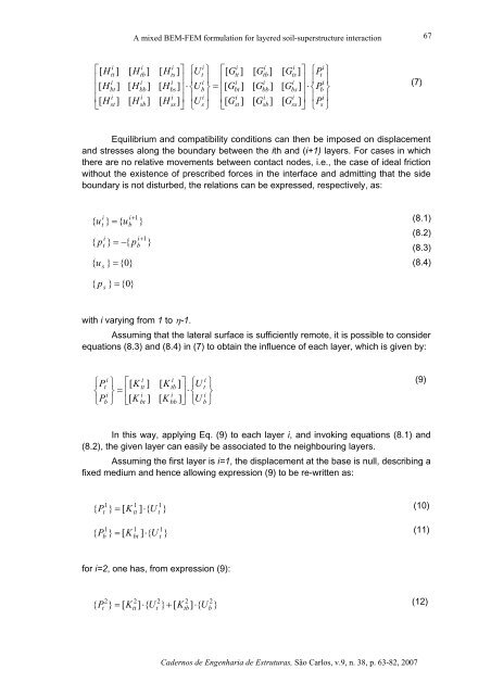
Equilibrium and compatibility conditions can then be imposed on displacement
and stresses along the boundary between the ith and (i+1) layers. For cases in which
there are no relative movements between contact nodes, i.e., the case of ideal friction
without the existence of prescribed forces in the interface and admitting that the side
boundary is not disturbed, the relations can be expressed, respectively, as:
{ u
i
t
{ p
} = { u
i
t
i+1
b
} = −{
p
{ u } = {0}
s
}
i+1
b
}
(8.1)
(8.2)
(8.3)
(8.4)
{ p } = {0}
s
with i varying from 1 to η-1.
Assuming that the lateral surface is sufficiently remote, it is possible to consider
equations (8.3) and (8.4) in (7) to obtain the influence of each layer, which is given by:
⎧
i
Pt
⎨ i
⎩Pb
⎫ ⎡[
K
⎬ = ⎢
⎭ ⎣[
K
i
tt
i
bt
]
]
[ K
[ K
i
tb
i
bb
] ⎤ ⎧U
⎥ ⋅ ⎨
] ⎦ ⎩U
i
t
i
b
⎫
⎬
⎭
(9)
In this way, applying Eq. (9) to each layer i, and invoking equations (8.1) and
(8.2), the given layer can easily be associated to the neighbouring layers.
Assuming the first layer is i=1, the displacement at the base is null, describing a
fixed medium and hence allowing expression (9) to be re-written as:
1
t
{ P
1
b
{ P
1 1
} = [ K ] ⋅{
U }
(10)
tt
t
1 1
} = [ K ] ⋅{
U }
(11)
bt
t
for i=2, one has, from expression (9):
2
t
{ P
2 2 2 2
} = [ K ] ⋅{
U } + [ K ] ⋅{
U }
(12)
tt
t
tb
b
Cadernos de Engenharia de Estruturas, São Carlos, v.9, n. 38, p. 63-82, 2007