Student Project Abstracts 2005 - Pluto - University of Washington

More documents

Recommendations

Info

40 CMDITR Review of Undergraduate Research Vol. 2 No. 1 Summer 2005x j x jkk k j x j j jkkx kmakes the approximation that q j q k = q j q k for j = k, that is, bathSimilar decomposition and approximations are applied to third orderves for σ x p j , σ y q j , and σ y p j .t to unity. The set of first order equations for the spin system aredt σ z = 2Ωσ y (5)dt σ x = −2εσ y + 2 jg j σ y q j (6)dt σ y = −2Ωσ z + 2εσ x − 2 jg j σ x q j . (7)ddt q j = p jµ j (8)ddt p j = −µ j ω 2 j q j + g j σ z . (9)ddt q2 j = 2 µ j p j q j s (10)2For simplicity ħ was set to unity. The set of first order equationsfor the spin system are(5)(6)(7)The bath terms evolve as(8)(9)(10)(11)(12)The first order spin terms depend on second order terms thatmix spin and bath degrees of freedom.(13)(14)(15)(16)(17)(18)There are eleven equations (2 first order, 6 mixed terms, and3 second order) for every bath oscillator and three for the spinterms that are required to describe motion of the system.ANALYSIS OF DYNAMICSIt has been demonstrated that the spin-boson system canevolve with many different patterns ranging from coherent oscillations,to incoherent relaxation and complete localizationdepending on various parameters. 3 The particular case studiedwith QHD is the asymmetric system, ε > Ω > 0 and watchinga system, starting with0.0010.010.010.10.0010.010.11101001000100001000001e+060 0.05 0.1 0.15 0.2 0.25P (υ)υCoupled Oscillators with ω > 9ε/4ω = 19ε/8ω = 10ε/40.010.11101001000100001000001e+060 0.05 0.1 0.15P (υ)υCoupled to Multiple OscillatorFigure 2: Power Spectra of Asymmetric Systems Coupled to Single Oscillatorconditions as Figure 1. The power spectra of the asymmetric systems show twoA high frequency oscillation, dependent on Ω and ε and the slower oscillation iFor an oscillator where ω is the natural frequency of the spin system more comoccurs.various parameters. 3 The particular case studied with QHD is the asymmetricand watching a system, starting with σ x (0) = 1, relax. The resulting equationssystem were then numerically integrating using a 4th-order Runge-Kutta algoconditions for the bath oscillators give minimal bath energy and uncertainty:q 2 j = 12µ j ω j . The other terms are all set initially to zero.A. Baths of Single OscillatorsFor the gas phase (no bath oscillators), the system can be solved analytically,sinusoidally in time with frequency.ω 0 = 2ε1 + Ω2ε 2This behavior changes when adding a single bath oscillator. If a bath oscillatooscillation frequency not close to the natural frequency of the spin system a nthan ω 0 , is added to the behavior of σ z . The closer ω j is to ω 0 the strongerthe lower the frequency of the added oscillation. This single oscillator respontime-domain of σ z in Figure 1 and the frequency domain in Figure 2.5relax. The resulting equationsof the spin-boson system were then numerically integratingusing a 4th-order Runge-Kutta algorithm. The initial conditionsfor the bath oscillators give minimal bath energy and uncertainty:0 0.05 0.1 0.15 0.2 0.25υω = 17ε/80.010.11101001000100001000000 0.05 0.1 0.15 0.2 0.25P (υ)υ0 0.05 0.1 0.15 0.2 0.25υCoupled Oscillators with ω > 9ε/4ω = 19ε/8ω = 10ε/40.010.11101001000100001000001e+060 0.05 0.1 0.15 0.2 0.25P (υ)υCoupled to Multiple Oscillatorsr Spectra of Asymmetric Systems Coupled to Single Oscillators, using the sameigure 1. The power spectra of the asymmetric systems show two major oscillations.cy oscillation, dependent on Ω and ε and the slower oscillation is dependent on ω.r where ω is the natural frequency of the spin system more complicated behaviorters. 3 The particular case studied with QHD is the asymmetric system, ε > Ω > 0system, starting with σ x (0) = 1, relax. The resulting equations of the spin-bosonen numerically integrating using a 4th-order Runge-Kutta algorithm. The initialthe bath oscillators give minimal bath energy and uncertainty: p 2 j = ω jµ j2 andhe other terms are all set initially to zero.f Single Oscillatorsphase (no bath oscillators), the system can be solved analytically, and σ z oscillatestime with frequency.ω 0 = 2ε1 + Ω2ε 2 (19)hanges when adding a single bath oscillator. If a bath oscillator is added with anency not close to the natural frequency of the spin system a new oscillation, lessed to the behavior of σ z . The closer ω j is to ω 0 the stronger the amplitude andrequency of the added oscillation. This single oscillator response is shown in theσ z in Figure 1 and the frequency domain in Figure 2.5and0.0010.010.111010010000 0.05 0.1 0.15 0.2 0P (υ)υ0.0010.010.11101001000100001000001e+060 0.05 0.1 0.15 0.2 0P (υ)υCoupled Oscillators with ω > 9ε/4ω = 19ε/8ω = 10ε/4Figure 2: Power Spectra of Asymmetric Systconditions as Figure 1. The power spectra of tA high frequency oscillation, dependent on ΩFor an oscillator where ω is the natural frequoccurs.various parameters. 3 The particular case studand watching a system, starting with σ x (0) =system were then numerically integrating usinconditions for the bath oscillators give minimq 2 j = 12µ j ω j . The other terms are all set initiaA. Baths of Single OscillatorsFor the gas phase (no bath oscillators), thesinusoidally in time with frequency.ω 0 =This behavior changes when adding a single boscillation frequency not close to the naturalthan ω 0 , is added to the behavior of σ z . Ththe lower the frequency of the added oscillattime-domain of σ z in Figure 1 and the frequThe other terms are all set initiallyto zero.BATHS OF SINGLE OSCILLATORSFor the gas phase (no bath oscillators), the system can besolved analytically, and0.0010.010.11101001000100001000000 0.05 0.1 0.15 0.2 0.25P (υ)υω = 7ε/4ω = 2ε/4ω = 17ε/80.010.11101001000100001000000 0.05 0.1 0.15 0.2 0.25P (υ)υ0.0010.010.11101001000100001000001e+060 0.05 0.1 0.15 0.2 0.25P (υ)υCoupled Oscillators with ω > 9ε/4ω = 19ε/8ω = 10ε/40.010.11101001000100001000001e+060 0.05 0.1 0.15 0.2 0.25P (υ)υCoupled to Multiple OscillatorsFigure 2: Power Spectra of Asymmetric Systems Coupled to Single Oscillators, using the sameconditions as Figure 1. The power spectra of the asymmetric systems show two major oscillations.A high frequency oscillation, dependent on Ω and ε and the slower oscillation is dependent on ω.For an oscillator where ω is the natural frequency of the spin system more complicated behavioroccurs.various parameters. 3 The particular case studied with QHD is the asymmetric system, ε > Ω > 0and watching a system, starting with σ x (0) = 1, relax. The resulting equations of the spin-bosonsystem were then numerically integrating using a 4th-order Runge-Kutta algorithm. The initialconditions for the bath oscillators give minimal bath energy and uncertainty: p 2 j = ω jµ j2 andq 2 j = 12µ j ω j . The other terms are all set initially to zero.A. Baths of Single OscillatorsFor the gas phase (no bath oscillators), the system can be solved analytically, and σ z oscillatessinusoidally in time with frequency.ω 0 = 2ε1 + Ω2ε 2 (19)This behavior changes when adding a single bath oscillator. If a bath oscillator is added with anoscillation frequency not close to the natural frequency of the spin system a new oscillation, lessthan ω 0 , is added to the behavior of σ z . The closer ω j is to ω 0 the stronger the amplitude andthe lower the frequency of the added oscillation. This single oscillator response is shown in thetime-domain of σ z in Figure 1 and the frequency domain in Figure 2.5oscillates sinusoidally in time withfrequency.(19)This behavior changes when adding a single bath oscillator.If a bath oscillator is added with an oscillation frequency notclose to the natural frequency of the spin system a new oscillation,less than0.0010.010.11101001000100001000001e+060 0.05 0.1 0.15 0.2 0.25P (υ)υCoupled Oscillators with ω < 9ε/4ω = 3ε/2ω = 7ε/4ω = 2ε/4ω = 17ε/81101P (υ)0.0010.010.11101001000100001000001e+060 0.05 0.1 0.15 0.2 0.25P (υ)υCoupled Oscillators with ω > 9ε/4ω = 19ε/8ω = 10ε/41101P (υ)Figure 2: Power Spectra of Asymmetric Systems Couconditions as Figure 1. The power spectra of the asymmA high frequency oscillation, dependent on Ω and ε andFor an oscillator where ω is the natural frequency of thoccurs.various parameters. 3 The particular case studied with Qand watching a system, starting with σ x (0) = 1, relax.system were then numerically integrating using a 4th-oconditions for the bath oscillators give minimal bathq 2 j = 12µ j ω j . The other terms are all set initially to zerA. Baths of Single OscillatorsFor the gas phase (no bath oscillators), the system casinusoidally in time with frequency.ω 0 = 2ε1 + Ω εThis behavior changes when adding a single bath oscilloscillation frequency not close to the natural frequencythan ω 0 , is added to the behavior of σ z . The closer ωthe lower the frequency of the added oscillation. Thistime-domain of σ z in Figure 1 and the frequency dom5is added to the behavior of0.0010.010.11101001000100001000001e+060 0.05 0.1 0.15 0.2 0.25P (υ)υCoupled Oscillators with ω < 9ε/4ω = 3ε/2ω = 7ε/4ω = 2ε/4ω = 17ε/80.010.11101001000100001000001e+060P (υ)0.0010.010.11101001000100001000001e+060 0.05 0.1 0.15 0.2 0.25P (υ)υCoupled Oscillators with ω > 9ε/4ω = 19ε/8ω = 10ε/40.010.11101001000100001000001e+060P (υ)Figure 2: Power Spectra of Asymmetric Systems Coupled toconditions as Figure 1. The power spectra of the asymmetric sA high frequency oscillation, dependent on Ω and ε and the sFor an oscillator where ω is the natural frequency of the spinoccurs.various parameters. 3 The particular case studied with QHD isand watching a system, starting with σ x (0) = 1, relax. The rsystem were then numerically integrating using a 4th-order Rconditions for the bath oscillators give minimal bath energyq 2 j = 12µ j ω j . The other terms are all set initially to zero.A. Baths of Single OscillatorsFor the gas phase (no bath oscillators), the system can be sosinusoidally in time with frequency.ω 0 = 2ε1 + Ω2ε 2This behavior changes when adding a single bath oscillator. Ioscillation frequency not close to the natural frequency of thethan ω 0 , is added to the behavior of σ z . The closer ω j is tothe lower the frequency of the added oscillation. This singletime-domain of σ z in Figure 1 and the frequency domain in5. The closer0.0010.010.11101001000100001000001e+060 0.05 0.1 0.15 0.2 0.25P (υ)υCoupled Oscillators with ω < 9ε/4ω = 3ε/2ω = 7ε/4ω = 2ε/4ω = 17ε/80.010.11101001000100001000001e+060 0.0P (υ)0.0010.010.11101001000100001000001e+060 0.05 0.1 0.15 0.2 0.25P (υ)υCoupled Oscillators with ω > 9ε/4ω = 19ε/8ω = 10ε/40.010.11101001000100001000001e+060 0.0P (υ)Figure 2: Power Spectra of Asymmetric Systems Coupled to Sconditions as Figure 1. The power spectra of the asymmetric systA high frequency oscillation, dependent on Ω and ε and the slowFor an oscillator where ω is the natural frequency of the spin syoccurs.various parameters. 3 The particular case studied with QHD is thand watching a system, starting with σ x (0) = 1, relax. The resusystem were then numerically integrating using a 4th-order Runconditions for the bath oscillators give minimal bath energy anq 2 j = 12µ j ω j . The other terms are all set initially to zero.A. Baths of Single OscillatorsFor the gas phase (no bath oscillators), the system can be solvsinusoidally in time with frequency.ω 0 = 2ε1 + Ω2ε 2This behavior changes when adding a single bath oscillator. If aoscillation frequency not close to the natural frequency of the spthan ω 0 , is added to the behavior of σ z . The closer ω j is to ωthe lower the frequency of the added oscillation. This single ostime-domain of σ z in Figure 1 and the frequency domain in Fig5is to0.0010.010.11101001000100001000001e+060 0.05 0.1 0.15 0.2 0.25P (υ)υCoupled Oscillators with ω < 9ε/4ω = 3ε/2ω = 7ε/4ω = 2ε/4ω = 17ε/80.010.11101001000100001000001e+060P (υ)0.0010.010.11101001000100001000001e+060 0.05 0.1 0.15 0.2 0.25P (υ)υCoupled Oscillators with ω > 9ε/4ω = 19ε/8ω = 10ε/40.010.11101001000100001000001e+060P (υ)Figure 2: Power Spectra of Asymmetric Systems Coupled toconditions as Figure 1. The power spectra of the asymmetric syA high frequency oscillation, dependent on Ω and ε and the sloFor an oscillator where ω is the natural frequency of the spin soccurs.various parameters. 3 The particular case studied with QHD isand watching a system, starting with σ x (0) = 1, relax. The resystem were then numerically integrating using a 4th-order Ruconditions for the bath oscillators give minimal bath energy aq 2 j = 12µ j ω j . The other terms are all set initially to zero.A. Baths of Single OscillatorsFor the gas phase (no bath oscillators), the system can be solsinusoidally in time with frequency.ω 0 = 2ε1 + Ω2ε 2This behavior changes when adding a single bath oscillator. Ifoscillation frequency not close to the natural frequency of thethan ω 0 , is added to the behavior of σ z . The closer ω j is to ωthe lower the frequency of the added oscillation. This single otime-domain of σ z in Figure 1 and the frequency domain in F5the stronger the amplitude and the lower the frequency ofthe added oscillation. This single oscillator response is shown inthe time-domain of0.0010.010.11101001000100001000001e+060 0.05 0.1 0.15 0.2 0.25P (υ)υCoupled Oscillators with ω < 9ε/4ω = 3ε/2ω = 7ε/4ω = 2ε/4ω = 17ε/80.010.11101001000100001000001e+060 0.05 0.1 0.15 0P (υ)υCoupled Oscillator with ω = 9ε/40.0010.010.11101001000100001000001e+060 0.05 0.1 0.15 0.2 0.25P (υ)υCoupled Oscillators with ω > 9ε/4ω = 19ε/8ω = 10ε/40.010.11101001000100001000001e+060 0.05 0.1 0.15 0P (υ)υCoupled to Multiple OscillatorsFigure 2: Power Spectra of Asymmetric Systems Coupled to Single Oscillators, uconditions as Figure 1. The power spectra of the asymmetric systems show two maA high frequency oscillation, dependent on Ω and ε and the slower oscillation is deFor an oscillator where ω is the natural frequency of the spin system more complioccurs.various parameters. 3 The particular case studied with QHD is the asymmetric systand watching a system, starting with σ x (0) = 1, relax. The resulting equations ofsystem were then numerically integrating using a 4th-order Runge-Kutta algorithconditions for the bath oscillators give minimal bath energy and uncertainty: pq 2 j = 12µ j ω j . The other terms are all set initially to zero.A. Baths of Single OscillatorsFor the gas phase (no bath oscillators), the system can be solved analytically, andsinusoidally in time with frequency.ω 0 = 2ε1 + Ω2ε 2This behavior changes when adding a single bath oscillator. If a bath oscillator isoscillation frequency not close to the natural frequency of the spin system a newthan ω 0 , is added to the behavior of σ z . The closer ω j is to ω 0 the stronger thethe lower the frequency of the added oscillation. This single oscillator response itime-domain of σ z in Figure 1 and the frequency domain in Figure 2.5in Figure 1 and the frequency domain inFigure 2.Adding single bath oscillators at frequencies, that are notclose to the spin system’s natural frequency, cause relativelysimple behavior in the system. This behavior of0.0010.010.11101001000100001000001e+060 0.05 0.1 0.15 0.2 0.25P (υ)υCoupled Oscillators with ω < 9ε/4ω = 3ε/2ω = 7ε/4ω = 2ε/4ω = 17ε/80.010.11101001000100001000001e+060P (υ)0.0010.010.11101001000100001000001e+060 0.05 0.1 0.15 0.2 0.25P (υ)υCoupled Oscillators with ω > 9ε/4ω = 19ε/8ω = 10ε/40.010.11101001000100001000001e+060P (υ)Figure 2: Power Spectra of Asymmetric Systems Coupledconditions as Figure 1. The power spectra of the asymmetrA high frequency oscillation, dependent on Ω and ε and thFor an oscillator where ω is the natural frequency of the soccurs.various parameters. 3 The particular case studied with QHand watching a system, starting with σ x (0) = 1, relax. Thsystem were then numerically integrating using a 4th-ordconditions for the bath oscillators give minimal bath eneq 2 j = 12µ j ω j . The other terms are all set initially to zero.A. Baths of Single OscillatorsFor the gas phase (no bath oscillators), the system can bsinusoidally in time with frequency.ω 0 = 2ε1 + Ω2ε 2This behavior changes when adding a single bath oscillatooscillation frequency not close to the natural frequency ofthan ω 0 , is added to the behavior of σ z . The closer ω j ithe lower the frequency of the added oscillation. This sintime-domain of σ z in Figure 1 and the frequency domain5coupled toa single bath oscillator off of0.0010.010.11101001000100001000001e+060 0.05 0.1 0.15 0.2P (υ)υCoupled Oscillators with ω < 9ε/4ω = 3ω = 7ω = 2ω = 170.0010.010.11101001000100001000001e+060 0.05 0.1 0.15 0.2P (υ)υCoupled Oscillators with ω > 9ε/4ω = 19ω = 10Figure 2: Power Spectra of Asymmetric Sconditions as Figure 1. The power spectraA high frequency oscillation, dependent onFor an oscillator where ω is the natural freoccurs.various parameters. 3 The particular case sand watching a system, starting with σ x (0system were then numerically integratingconditions for the bath oscillators give miq 2 j = 12µ j ω j . The other terms are all set inA. Baths of Single OscillatorsFor the gas phase (no bath oscillators), tsinusoidally in time with frequency.ω 0This behavior changes when adding a singoscillation frequency not close to the natuthan ω 0 , is added to the behavior of σ z .the lower the frequency of the added osciltime-domain of σ z in Figure 1 and the frecan be described as energy pass-≈ (σ x q j − σ x q j ) kg k q k + g j σ x (q 2 j − q j 2 ) + q j kg k σ x q k (4)p in eq 4 makes the approximation that q j q k = q j q k for j = k, that is, bathcoupled. Similar decomposition and approximations are applied to third orderderivatives for σ x p j , σ y q j , and σ y p j .¯h was set to unity. The set of first order equations for the spin system areddt σ z = 2Ωσ y (5)ddt σ x = −2εσ y + 2 jg j σ y q j (6)ddt σ y = −2Ωσ z + 2εσ x − 2 jg j σ x q j . (7)volve asddt q j = p jµ j (8)ddt p j = −µ j ω 2 j q j + g j σ z . (9)ddt q2 j = 2 µ j p j q j s (10)2σ x q j − σ x q j )kg k q k + g j σ x (q 2 j − q j 2 ) + q j kg k σ x q k (4)4 makes the approximation that q j q k = q j q k for j = k, that is, bath. Similar decomposition and approximations are applied to third ordertives for σ x p j , σ y q j , and σ y p j .set to unity. The set of first order equations for the spin system areddt σ z = 2Ωσ y (5)ddt σ x = −2εσ y + 2 jg j σ y q j (6)ddt σ y = −2Ωσ z + 2εσ x − 2 jg j σ x q j . (7)sddt q j = p jµ j (8)ddt p j = −µ j ω 2 j q j + g j σ z . (9)ddt q2 j = 2 µ j p j q j s (10)2kkeq 4 makes the approximation that q j q k = q j q k for j = k, that is, bathled. Similar decomposition and approximations are applied to third ordervatives for σ x p j , σ y q j , and σ y p j .s set to unity. The set of first order equations for the spin system areddt σ z = 2Ωσ y (5)ddt σ x = −2εσ y + 2 jg j σ y q j (6)ddt σ y = −2Ωσ z + 2εσ x − 2 jg j σ x q j . (7)asddt q j = p jµ j (8)ddt p j = −µ j ω 2 j q j + g j σ z . (9)ddt q2 j = 2 µ j p j q j s (10)2≈ (σ x q j − σ x q j )kg k q k + g j σ x (q 2 j − q j 2 ) + q j kg k σ x q k (4)p in eq 4 makes the approximation that q j q k = q j q k for j = k, that is, bathcoupled. Similar decomposition and approximations are applied to third orderderivatives for σ x p j , σ y q j , and σ y p j .¯h was set to unity. The set of first order equations for the spin system areddt σ z = 2Ωσ y (5)ddt σ x = −2εσ y + 2 jg j σ y q j (6)ddt σ y = −2Ωσ z + 2εσ x − 2 jg j σ x q j . (7)volve asddt q j = p jµ j (8)ddt p j = −µ j ω 2 j q j + g j σ z . (9)ddt q2 j = 2 µ j p j q j s (10)2ddt p jq j s = p2 j µ j − µ j ω 2 j q 2 j + g j σ z q j (11)ddt p2 j = −2µ j ω 2 j p j q j s + 2g j σ z p j . (12)terms depend on second order terms that mix spin and bath degrees of freedom.ddt σ zq j = 2Ωσ y q j + 1 µ j σ z p j (13)ddt σ zp j = 2Ωσ y p j − µ j ω 2 j σ z q j + g j (14)ddt σ xq j = −2εσ y q j + 1 µ j σ x p j +2g j σ y (q 2 j − q j 2 )+2q j kg k σ y q k +2(σ y q j − σ y q j ) kg k q k (15)ddt σ xp j = −2εσ y p j − µ j ω 2 j σ x q j +2(σ y p j − σ y p j ) kg k q k +2p j kg k σ y q k +2g j σ y (p j q j s − p j q j ) (16)ddt σ yq j = −2Ωσ z q j + 2εσ x q j + 1 µ j σ y p j −2g j σ x (q 2 j − q j 2 )−2q j kg k σ x q k −2(σ x q j − σ x q j ) kg k q k (17)ddt σ yp j = −2Ωσ z p j + 2εσ x p j − µ j ω 2 j σ y q j ddt p jq j s = p2 j µ j − µ j ω 2 j q 2 j + g j σ z q j (11)ddt p2 j = −2µ j ω 2 j p j q j s + 2g j σ z p j . (12)terms depend on second order terms that mix spin and bath degrees of freedom.ddt σ zq j = 2Ωσ y q j + 1 µ j σ z p j (13)ddt σ zp j = 2Ωσ y p j − µ j ω 2 j σ z q j + g j (14)ddt σ xq j = −2εσ y q j + 1 µ j σ x p j +2g j σ y (q 2 j − q j 2 )+2q j kg k σ y q k +2(σ y q j − σ y q j ) kg k q k (15)ddt σ xp j = −2εσ y p j − µ j ω 2 j σ x q j +2(σ y p j − σ y p j ) kg k q k +2p j kg k σ y q k +2g j σ y (p j q j s − p j q j ) (16)ddt σ yq j = −2Ωσ z q j + 2εσ x q j + 1 µ j σ y p j −2g j σ x (q 2 j − q j 2 )−2q j kg k σ x q k −2(σ x q j − σ x q j ) kg k q k (17)ddt p jq j s = p2 j µ j − µ j ω 2 j q 2 j + g j σ z q j (11)ddt p2 j = −2µ j ω 2 j p j q j s + 2g j σ z p j . (12)in terms depend on second order terms that mix spin and bath degrees of freedom.ddt σ zq j = 2Ωσ y q j + 1 µ j σ z p j (13)ddt σ zp j = 2Ωσ y p j − µ j ω 2 j σ z q j + g j (14)ddt σ xq j = −2εσ y q j + 1 µ j σ x p j +2g j σ y (q 2 j − q j 2 )+2q j kg k σ y q k +2(σ y q j − σ y q j ) kg k q k (15)ddt σ xp j = −2εσ y p j − µ j ω 2 j σ x q j +2(σ y p j − σ y p j ) kg k q k +2p j kg k σ y q k +2g j σ y (p j q j s − p j q j ) (16)ddt σ yq j = −2Ωσ z q j + 2εσ x q j + 1 µ j σ y p j −2g j σ x (q 2 j − q j 2 )−2q j kg k σ x q k −2(σ x q j − σ x q j ) kg k q k (17)j y j j s j jddt σ yq j = −2Ωσ z q j + 2εσ x q j + 1 µ j σ y p j −2g j σ x (q 2 j − q j 2 )−2q j kg k σ x q k −2(σ x q j − σ x q j ) kg k q k ddt σ yp j = −2Ωσ z p j + 2εσ x p j − µ j ω 2 j σ y q j −2(σ x p j − σ x p j ) kg k q k −2p j kg k σ x q k −2σ x (p j q j s − p j q j )There are eleven equations (2 first order, 6 mixed terms, and 3 second order) for every bathand three for the spin terms that are required to describe motion of the system.IV.Analysis of DynamicsIt has been demonstrated that the spin-boson system can evolve with many differenranging from coherent oscillations, to incoherent relaxation and complete localization dep30.0010.010.11101001000100001000000 0.05 0.1 0.15 0.2 0.25P (υ)υω = 3ε/2ω = 7ε/4ω = 2ε/4ω = 17ε/80.010.11101001000100001000000 0.05 0.1 0.15 0.2P (υ)υ0.0010.010.11101001000100001000001e+060 0.05 0.1 0.15 0.2 0.25P (υ)υCoupled Oscillators with ω > 9ε/4ω = 19ε/8ω = 10ε/40.010.11101001000100001000001e+060 0.05 0.1 0.15 0.2P (υ)υCoupled to Multiple OscillatorsFigure 2: Power Spectra of Asymmetric Systems Coupled to Single Oscillators, uconditions as Figure 1. The power spectra of the asymmetric systems show two majoA high frequency oscillation, dependent on Ω and ε and the slower oscillation is depFor an oscillator where ω is the natural frequency of the spin system more complicoccurs.various parameters. 3 The particular case studied with QHD is the asymmetric systeand watching a system, starting with σ x (0) = 1, relax. The resulting equations of tsystem were then numerically integrating using a 4th-order Runge-Kutta algorithmconditions for the bath oscillators give minimal bath energy and uncertainty: p 2 jq 2 j = 12µ j ω j . The other terms are all set initially to zero.A. Baths of Single OscillatorsFor the gas phase (no bath oscillators), the system can be solved analytically, andsinusoidally in time with frequency.ω 0 = 2ε1 + Ω2ε 2This behavior changes when adding a single bath oscillator. If a bath oscillator is aoscillation frequency not close to the natural frequency of the spin system a new othan ω 0 , is added to the behavior of σ z . The closer ω j is to ω 0 the stronger the athe lower the frequency of the added oscillation. This single oscillator response istime-domain of σ z in Figure 1 and the frequency domain in Figure 2.5QUANTIZED HAMILTON DYNAMICS APPLIED TO CONDENSED PHASE SPIN-RELAXATION
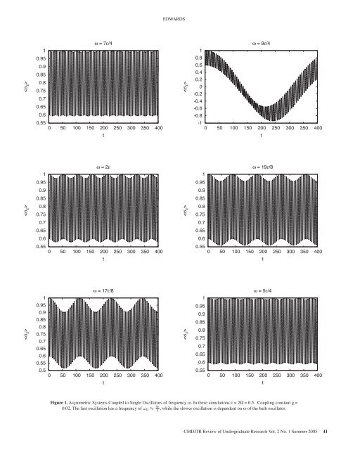
EDWARDSω = 7ε/410.950.90.850.80.750.70.650.60.550 50 100 150 200 250 300 350 400tω = 9ε/410.80.60.40.20-0.2-0.4-0.6-0.8-10 50 100 150 200 250 300 350 400tω = 7ε/4100 150 200 250 300 350 400tω = 2ε100 150 200 250 300 350 400tω = 17ε/8100 150 200 250 300 350 400t10.950.90.850.80.750.70.650.60.5510.950.90.850.80.750.70.650.60.5510.80.60.40.20-0.2-0.4-0.6-0.8ω = 9ε/4-10 50 100 150 200 250 300 350 400t10 50 100 0.95 150 200 250 300 350 4000.90.850.80.750.70.650.6ω = 19ε/80.550 50 100 150 200 250 300 350 400t10.950.90.850.80.750.70.65ω = 2εtω = 17ε/8ω = 5ε/40.50.60 50 100 150 200 250 300 350 4000.550 50 100 150 200 250 300 350 400ttω = 19ε/810.950.90.850.80.750.70.650.60.550 50 100 150 200 250 300 350 400tω = 5ε/410.950.90.850.80.750.70.650.60.550 50 100 150 200 250 300 350 400ttric Systems Coupled to Figure Single 1. Asymmetric OscillatorsSystems of frequency Coupled ω. to Single In these Oscillators simulations of frequency ω. In these simulations ε = 2Ω = 0.5. Coupling constant g =upling constant g = 0.02. The 0.02. fast The oscillation fast has has a frequency a of ω 0 ≈ 9ε4 , while the slower oscillation is dependent on ω of the bath oscillator.ion is dependent on ω of the bath oscillator.Figure 1: Asymmetric Systems Coupled to Single Oscillators of frequency ω. In these simulationsε = 2Ω = 0.5 . Coupling constant g = 0.02. The fast oscillation has a frequency of ω 0 ≈ 9ε4 , whilethe slower oscillation is dependent on ω of the bath oscillator.4CMDITR Review of Undergraduate Research Vol. 2 No. 1 Summer 2005 41
Page 2 and 3: The material is based upon work sup
Page 4 and 5: TABLE OF CONTENTSSynthesis of Dendr
Page 6 and 7: 6 CMDITR Review of Undergraduate Re
Page 8 and 9: SYNTHESIS OF DENDRIMER BUILDING BLO
Page 10 and 11: throughout the work period. Five su
Page 12 and 13: 12 CMDITR Review of Undergraduate R
Page 14 and 15: BARIUM TITANATE DOPED SOL-GEL FOR E
Page 16 and 17: BARIUM TITANATE DOPED SOL-GEL FOR E
Page 18 and 19: SYNTHESIS OF NORBORNENE MONOMER OF
Page 20: 20 CMDITR Review of Undergraduate R
Page 23 and 24: using different reaction conditions
Page 25 and 26: Synthesis of Nonlinear Optical-Acti
Page 27 and 28: quality of the XRD structures wasca
Page 29 and 30: Behavioral Properties of Colloidal
Page 32 and 33: Transmission electron microscopy ha
Page 36 and 37: areorient themselves with the elect
Page 38 and 39: Fabry-Perot modulators with electro
Page 42 and 43: QUANTIZED HAMILTON DYNAMICS APPLIED
Page 46 and 47: INVESTIGATING NEW CLADDING AND CORE
Page 48 and 49: Dr. Robert NorwoodChris DeRoseAmir
Page 50 and 51: SYNTHESIS OF TPD-BASED COMPOUNDS FO
Page 52 and 53: SYNTHESIS OF TPD-BASED COMPOUNDS FO
Page 54 and 55: OPTIMIZING HYBRID WAVEGUIDESpropaga
Page 56 and 57: At closer spaces the second undesir
Page 58 and 59: SYNTHESIS AND ANALYSIS OF THIOL-STA
Page 62 and 63: QUINOXALINE-CONTAINING POLYFLUORENE
Page 64 and 65: QUINOXALINE-CONTAINING POLYFLUORENE
Page 68 and 69: SYNTHESIS OF DENDRON-FUNCTIONALIZED
Page 72 and 73: BUILDING AN OPTICAL OXIMETER TO MEA
Page 78 and 79: TOWARD MOLECULAR RESOLUTION C-AFM W
Page 80 and 81: TOWARD MOLECULAR RESOLUTION C-AFM W
Page 82 and 83: SYNTHESIS AND CHARACTERIZATION OF E
Page 84 and 85: My name is Aaron Montgomery and I a
Page 86 and 87: 1,1-DIPHENYL-2,3,4,5-TETRAKIS(9,9-D
Page 88 and 89: 1,1-DIPHENYL-2,3,4,5-TETRAKIS(9,9-D
Page 90 and 91:
EFFECTS OF SURFACE CHEMISTRY ON CAD
Page 92 and 93:
EFFECTS OF SURFACE CHEMISTRY ON CAD
Page 94 and 95:
94 CMDITR Review of Undergraduate R
Page 96 and 97:
SYNTHESIS OF A POLYENE EO CHROMOPHO
Page 98 and 99:
SYNTHESIS OF A POLYENE EO CHROMOPHO
Page 102 and 103:
102 CMDITR Review of Undergraduate
Page 104 and 105:
CHARACTERIZATION OF THE MOLECULAR P
Page 106 and 107:
Page 108 and 109:
OPTIMIZATION OF SEMICONDUCTOR NANOP
Page 110 and 111:
OPTIMIZATION OF SEMICONDUCTOR NANOP
Page 112 and 113:
CHARACTERIZATION OF THE PHOTODECOMP
Page 114 and 115:
Page 116 and 117:
ELECTROLUMINESCENT PROPERTIES OF OR
Page 118 and 119:
Page 120 and 121:
DETERMINATION OF MOLECULAR ORIENTAT
Page 122 and 123:
DETERMINATION OF MOLECULAR ORIENTAT
Page 124 and 125:
HYDROGEL MATERIALS FOR TWO-PHOTON M
Page 126 and 127:
HYDROGEL MATERIALS FOR TWO-PHOTON M
Page 128 and 129:
THE DESIGN OF A FLUID DELIVERY SYST
Page 130:
THE DESIGN OF A FLUID DELIVERY SYST
show all

Student Project Abstracts 2005 - Pluto - University of Washington

You also want an ePaper? Increase the reach of your titles

Delete template?

Save as template?