- Page 1:
User’s Guide December 22, 2011 Si
- Page 4 and 5:
PTI RAW File Load Options .........
- Page 6 and 7:
Custom Case Information Display ...
- Page 8 and 9:
Line Per Unit Impedance Calculator
- Page 10 and 11:
Bus View Display ..................
- Page 12 and 13:
Data View .........................
- Page 14 and 15:
Switched Shunt Fields on Onelines .
- Page 16 and 17:
Oneline Animation .................
- Page 18 and 19:
Tapping Transmission Lines.........
- Page 20 and 21:
Tutorial: Contingency Analysis - Pa
- Page 22 and 23:
Determining Set of Active Inequalit
- Page 24 and 25:
ATC Analysis Methods: Single Linear
- Page 26 and 27:
SaveCase Function (version 9) .....
- Page 28 and 29:
Tutorial: Inserting a Transformer P
- Page 30 and 31:
Introduction to PowerWorld Simulato
- Page 32 and 33:
Distributed Computing Distributed c
- Page 34 and 35:
The following are new oneline diagr
- Page 36 and 37:
Added new Custom Monitoring to the
- Page 38 and 39:
control and is required to meet the
- Page 40 and 41:
economic range. Generators that are
- Page 42 and 43:
Bus can be specified by number [BUS
- Page 44 and 45:
Contact Information PowerWorld Corp
- Page 46 and 47:
Example Windows Styles ©2011 Power
- Page 48 and 49:
Edit Mode Introduction The Edit Mod
- Page 50 and 51:
Script Mode Introduction The Script
- Page 52 and 53:
Custom and Memo Display The Custom
- Page 54 and 55:
Ribbons User Interface PowerWorld's
- Page 56 and 57:
on Title Bar Applicati on Button Cl
- Page 58 and 59:
Add Ons Ribbon Tab The Add Ons ribb
- Page 60 and 61:
Topology Processing Ribbon Group To
- Page 62 and 63:
Case Data Ribbon Group Difference F
- Page 64 and 65:
The Open Windows Menu provides a co
- Page 66 and 67:
Clipboard Ribbon Group The Clipboar
- Page 68 and 69:
Formatting Ribbon Group The Formatt
- Page 70 and 71:
Individual Insert Ribbon Group The
- Page 72 and 73:
Quick Insert Ribbon Group The Quick
- Page 74 and 75:
Select Ribbon Group The Select ribb
- Page 76 and 77:
Click on this button to open the di
- Page 78 and 79:
GIS Tools Menu Provides access to m
- Page 80 and 81:
Save View Choose this option to ope
- Page 82 and 83:
Options Ribbon Tab The Options ribb
- Page 84 and 85:
Solution Options Quick Menu The Sol
- Page 86 and 87:
For more detailed help see the Othe
- Page 88 and 89:
©2011 PowerWorld Corporation 60
- Page 90 and 91:
Determine Path Distances to Buses:
- Page 92 and 93:
Power Flow Tools Ribbon Group The m
- Page 94 and 95:
Usually, a flat start should be use
- Page 96 and 97:
Redraws (refreshes) each of the ope
- Page 98 and 99:
Application File Menu The Applicati
- Page 100 and 101:
use, however Simulator does store t
- Page 102 and 103:
When using the Present Topological
- Page 104 and 105:
GE EPC File Load Options The GE EPC
- Page 106 and 107:
PTI RAW File Load Options This dial
- Page 108 and 109:
Opening a Oneline Diagram Simulator
- Page 110 and 111:
Recently Opened Cases A numbered li
- Page 112 and 113:
Building a New Oneline This option
- Page 114 and 115:
Saving a Oneline Select Save Onelin
- Page 116 and 117:
Generator Capability Curves Format
- Page 118 and 119:
Cross-compound is a generator archi
- Page 120 and 121:
Interface Data Format (*.inf) These
- Page 122 and 123:
tGzer, tBzer zero sequence line shu
- Page 124 and 125:
Saving Images as Jpegs Simulator ca
- Page 126 and 127:
Working With GE EPC Files PowerWorl
- Page 128 and 129:
PSLF supports up to 8 owners per br
- Page 130 and 131:
In Simulator, each bus can be optio
- Page 132 and 133:
PowerWorld Project Initialization S
- Page 134 and 135:
The *.pwp file type will now be rec
- Page 136 and 137:
Create Project Dialog The Create Pr
- Page 138 and 139:
Opening an Existing Project To open
- Page 140 and 141:
Fields Pane ©2011 PowerWorld Corpo
- Page 142 and 143:
Model Explorer: Fields Pane The Fie
- Page 144 and 145:
©2011 PowerWorld Corporation 116
- Page 146 and 147:
Configuring the Case Information Di
- Page 148 and 149:
Also note that fields that the Gree
- Page 150 and 151:
Custom Field Descriptions Custom Fi
- Page 152 and 153:
Custom Field Description Dialog The
- Page 154 and 155:
Calculated Fields Calculated fields
- Page 156 and 157:
Case Information Customizations Dis
- Page 158 and 159:
Moves the case information display
- Page 160 and 161:
Case Information Displays: Using Ce
- Page 162 and 163:
Case Information Displays: Finding
- Page 164 and 165:
HTML Table Format Dialog The Table
- Page 166 and 167:
Set contains actions for setting da
- Page 168 and 169:
Case Information Toolbar: Copy, Pas
- Page 170 and 171:
Case Information Toolbar: Filtering
- Page 172 and 173:
Case Information Toolbar: Geo Data
- Page 174 and 175:
Case Information Toolbar: Save Auxi
- Page 176 and 177:
Case Information Toolbar: Records M
- Page 178 and 179:
Case Information Toolbar: Set, Togg
- Page 180 and 181:
Case Information Filterbar On the M
- Page 182 and 183:
Advanced Filtering Filtering by are
- Page 184 and 185:
epresent the filter. If the use of
- Page 186 and 187:
Advanced Filtering: Advanced The Ad
- Page 188 and 189:
Advanced Filtering: Device The Adva
- Page 190 and 191:
Custom Expressions Simulator allows
- Page 192 and 193:
Custom String Expressions Simulator
- Page 194 and 195:
MAX Maximum value ©2011 PowerWorld
- Page 196 and 197:
Model Expressions Model Expressions
- Page 198 and 199:
Similarly, normally you may only en
- Page 200 and 201:
Find Dialog Basics Many times when
- Page 202 and 203:
Search for Text Dialog This dialog
- Page 204 and 205:
Model Filters Display and Dialog Mo
- Page 206 and 207:
Entering a Range of Numbers On a nu
- Page 208 and 209:
Copying Simulator Data to and from
- Page 210 and 211:
Key Fields Key fields are necessary
- Page 212 and 213:
Required Fields Required fields are
- Page 214 and 215:
Contour Column Type Color Map Choos
- Page 216 and 217:
Grid Metrics Dialog The grid metric
- Page 218 and 219:
The uppermost part of the dialog bo
- Page 220 and 221:
Available SubData : lists the SubDa
- Page 222 and 223:
When creating a new geographic data
- Page 224 and 225:
There are two choices of Field Look
- Page 226 and 227:
Stack Level An object's stack level
- Page 228 and 229:
Geographic Data View Styles Each ge
- Page 230 and 231:
Custom Case Information Display To
- Page 232 and 233:
©2011 PowerWorld Corporation 204
- Page 234 and 235:
©2011 PowerWorld Corporation 206
- Page 236 and 237:
Show Fields Secondary This mode is
- Page 238 and 239:
User-Defined Case Information Displ
- Page 240 and 241:
Case Description The Case Descripti
- Page 242 and 243:
Case Summary The Case Summary Displ
- Page 244 and 245:
Power Flow List The Power Flow List
- Page 246 and 247:
Quick Power Flow List The Quick Pow
- Page 248 and 249:
Area Display The Area Display house
- Page 250 and 251:
Zone Display The Zone Display provi
- Page 252 and 253:
Far Area Name, Far Number, Far Name
- Page 254 and 255:
Super Area Display The Super Area D
- Page 256 and 257:
Bus Display The Bus Display present
- Page 258 and 259:
Remotely Regulated Bus Display The
- Page 260 and 261:
Substation Records Display The Subs
- Page 262 and 263:
Minimum and maximum allowable real
- Page 264 and 265:
Generator/Load Cost Models The Gene
- Page 266 and 267:
Parameters used to model the cost c
- Page 268 and 269:
An informational field that can be
- Page 270 and 271:
Unit Type An informational field th
- Page 272 and 273:
Load Benefit Models Display The Loa
- Page 274 and 275:
Line and Transformer Display The Li
- Page 276 and 277:
Merge Line Terminals A transmission
- Page 278 and 279:
200% and 300%. Also series caps and
- Page 280 and 281:
Of particular interest on the dialo
- Page 282 and 283:
section line going to the to bus an
- Page 284 and 285:
For an LTC transformer, this is the
- Page 286 and 287:
Renumber Star Buses... This option
- Page 288 and 289:
DC Lines Display The DC Line Displa
- Page 290 and 291:
Switched Shunt Display The Switched
- Page 292 and 293:
Interface Display The Interface Dis
- Page 294 and 295:
Nomogram Display The Nomogram Displ
- Page 296 and 297:
Indicates the degree to which switc
- Page 298 and 299:
entering changes directly in the ta
- Page 300 and 301:
MAX SHUNT DEC The participation fac
- Page 302 and 303:
Island Display The Island Display p
- Page 304 and 305:
Transaction Dialog The Transaction
- Page 306 and 307:
Owner Data Information Display The
- Page 308 and 309:
Owned Bus Records Display The Owned
- Page 310 and 311:
Owned Generator Records Display The
- Page 312 and 313:
Jacobian Display The Jacobian displ
- Page 314 and 315:
Bus Information (Edit Mode) This di
- Page 316 and 317:
Size Specifies the vertical axis of
- Page 318 and 319:
Bus Name Name of the bus Bus Number
- Page 320 and 321:
Bus Voltage Regulating Devices Dial
- Page 322 and 323:
of the substation object. Use the W
- Page 324 and 325:
Total Load MW or MVAR in the substa
- Page 326 and 327:
There are six additional areas of i
- Page 328 and 329:
Include Suffix If the Include Suffi
- Page 330 and 331:
Generator Options: Power and Voltag
- Page 332 and 333:
For Constant mode, Max Mvar Output
- Page 334 and 335:
The cost shift and cost multiplier
- Page 336 and 337:
Generator Options: Owners, Area, Zo
- Page 338 and 339:
Set Generator Participation Factors
- Page 340 and 341:
Generator Reactive Power Capability
- Page 342 and 343:
Substation Number, Substation Name
- Page 344 and 345:
Load Options: OPF Load Dispatch Thi
- Page 346 and 347:
Anchored If the Anchored checkbox i
- Page 348 and 349:
Branch Options (Edit Mode) The Bran
- Page 350 and 351:
The Memo section of the dialog is s
- Page 352 and 353:
Branch Options: Parameters The Para
- Page 354 and 355:
Line Per Unit Impedance Calculator
- Page 356 and 357:
values section. The characteristic
- Page 358 and 359:
Frequency: Frequency of the system
- Page 360 and 361:
GMR Geometric mean radius given in
- Page 362 and 363:
The distributed series impedance an
- Page 364 and 365:
Where: LimAmp Limit in Amperes LimM
- Page 366 and 367:
dialog allows changing the control
- Page 368 and 369:
Transformer AVR Dialog The Transfor
- Page 370 and 371:
Branch Options: Series Capacitor Th
- Page 372 and 373:
Save Saves any modifications but do
- Page 374 and 375:
AC Line MVA Flow Magnitude of MVA f
- Page 376 and 377:
Transformer Field Options Dialog Tr
- Page 378 and 379:
DC Transmission Line Options This d
- Page 380 and 381:
specify power flow at the inverter
- Page 382 and 383:
DC Line Options: Inverter Parameter
- Page 384 and 385:
DC Line Options: OPF This page is u
- Page 386 and 387:
Specifies the DC control mode for e
- Page 388 and 389:
Multi-Terminal DC Record Informatio
- Page 390 and 391:
Multi-Terminal DC Converter Informa
- Page 392 and 393:
Multi-Terminal DC Line Information
- Page 394 and 395:
dialog allows changing the control
- Page 396 and 397:
Transformers Bases and Impedances D
- Page 398 and 399:
Transformer AVR Dialog The Transfor
- Page 400 and 401:
Transformer Mvar Control Dialog The
- Page 402 and 403:
Transformer Phase Shifting Dialog T
- Page 404 and 405:
Transformer Field Options Dialog Tr
- Page 406 and 407:
Three Winding Transformer Informati
- Page 408 and 409:
Switched Shunt Information (Edit Mo
- Page 410 and 411:
MW components, and this field will
- Page 412 and 413:
Include Suffix If the Include Suffi
- Page 414 and 415:
©2011 PowerWorld Corporation Custo
- Page 416 and 417:
Each bus is associated with an Owne
- Page 418 and 419:
Bus Voltage Regulating Devices Dial
- Page 420 and 421:
©2011 PowerWorld Corporation Buses
- Page 422 and 423:
Read-only check-box that indicates
- Page 424 and 425:
Designates whether or not the gener
- Page 426 and 427:
Generator Options: Costs The Costs
- Page 428 and 429:
Generator Information: OPF The fiel
- Page 430 and 431:
Load Information (Run Mode) The Loa
- Page 432 and 433:
Branch Information Dialog (Run Mode
- Page 434 and 435:
Maximum MVA Flow The largest MVA fl
- Page 436 and 437:
Transformer AVR Dialog The Transfor
- Page 438 and 439:
Transformer Mvar Control Dialog The
- Page 440 and 441:
Transformer Phase Shifting Dialog T
- Page 442 and 443:
Transformer Impedance Correction Ta
- Page 444 and 445:
Nominal Mvar ©2011 PowerWorld Corp
- Page 446 and 447:
Zone Information (Run Mode) This di
- Page 448 and 449:
Labels Using Labels for Identificat
- Page 450 and 451:
ATC Extra Monitors ATC Extra Monito
- Page 452 and 453:
Latitude/Longitude and UTM Coordina
- Page 454 and 455:
Area Information The Area Informati
- Page 456 and 457:
Area Information: Buses The Area Bu
- Page 458 and 459:
Area Information: Loads The Area Lo
- Page 460 and 461:
Area Information: Info/Interchange
- Page 462 and 463:
Area Information: Tie Lines The Tie
- Page 464 and 465:
Area Information: Custom The Custom
- Page 466 and 467:
Include Suffix If the Include Suffi
- Page 468 and 469:
generation in the super area by rat
- Page 470 and 471:
Super Area Field Information Super
- Page 472 and 473:
Interface Information The Interface
- Page 474 and 475:
Interface Element Information The I
- Page 476 and 477:
Interface Pie Chart Information Dia
- Page 478 and 479:
Nomogram Information Dialog The Nom
- Page 480 and 481:
Injection Group Overview An injecti
- Page 482 and 483:
Auto Insert Injection Groups Many t
- Page 484 and 485:
Deleting Injection Groups To delete
- Page 486 and 487:
Indicates the degree to which switc
- Page 488 and 489:
entering changes directly in the ta
- Page 490 and 491:
Participation Points Overview A par
- Page 492 and 493:
MAX SHUNT DEC The participation fac
- Page 494 and 495:
Add Participation Points Dialog The
- Page 496 and 497:
Transaction Dialog The Transaction
- Page 498 and 499:
Bus View Display The Bus View Displ
- Page 500 and 501:
Open Multiple Bus Views This option
- Page 502 and 503:
Labels Using Labels for Identificat
- Page 504 and 505:
ATC Scenarios ATC Scenario change r
- Page 506 and 507:
Difference Flows The Difference Flo
- Page 508 and 509:
Using Difference Flows To use the D
- Page 510 and 511:
Present Topological Differences fro
- Page 512 and 513:
Auxiliary Files PowerWorld has inco
- Page 514 and 515:
Script Command Execution Dialog The
- Page 516 and 517:
Script Section The SCRIPT section b
- Page 518 and 519:
OpenCase ("filename ", AppendCa se
- Page 520 and 521:
LOAD MW [P,Q] BUS GEN FACTOR [P] (m
- Page 522 and 523:
DeleteIncludingContents(objecttype,
- Page 524 and 525:
different objects and save these in
- Page 526 and 527:
Use this action to treat the remain
- Page 528 and 529:
UseAreaZone : An optional parameter
- Page 530 and 531:
GenForceLDC_RCC(filter); Use this a
- Page 532 and 533:
[start] : same as the starting plac
- Page 534 and 535:
OWNER: Means that the elements will
- Page 536 and 537:
"OnelineName": The name of the onel
- Page 538 and 539:
RenumberMSLineDummyBuses ("filename
- Page 540 and 541:
Use this action to merge a set of b
- Page 542 and 543:
[value1, …, value8]: The set of r
- Page 544 and 545:
CalculateTLRMultipleElement (TypeEl
- Page 546 and 547:
CalculateLODF([BRANCH nearbusnum fa
- Page 548 and 549:
[AREA num], [AREA "name"], [AREA "l
- Page 550 and 551:
SetSensitivitiesAtOutOfServiceToClo
- Page 552 and 553:
"filename2" The filename of the aux
- Page 554 and 555:
DiffFlowMode(diffmode); Call this a
- Page 556 and 557:
CTGWriteResultsAndOptions("filename
- Page 558 and 559:
©2011 PowerWorld Corporation 530
- Page 560 and 561:
ATCIncreaseTransferBy(amount); Call
- Page 562 and 563:
Script PV Related Actions The follo
- Page 564 and 565:
Script QV Related Actions The follo
- Page 566 and 567:
Script Topology Processing Related
- Page 568 and 569:
Script Transient Stability Related
- Page 570 and 571:
Loads transient stability data in t
- Page 572 and 573:
Data Argument List The DATA argumen
- Page 574 and 575:
note that blank rows are ignored Ar
- Page 576 and 577:
Data List After the data argument l
- Page 578 and 579:
Data ATC_Options RLScenarioName GSc
- Page 580 and 581:
Data ATCScenario TransferLimiter Th
- Page 582 and 583:
Data AuxFileExportFormatData DataBl
- Page 584 and 585:
Data BGCalculatedField Condition Ca
- Page 586 and 587:
Data BusViewFormOptions BusViewBusF
- Page 588 and 589:
Data Contingency CTGElementAppend T
- Page 590 and 591:
Overview topic. Note: bus# values m
- Page 592 and 593:
as close to the desired amount with
- Page 594 and 595:
BAMP "1 3 1 1 FROMTO" 271.94031 398
- Page 596 and 597:
Data CTGElementBlock CTGElement Thi
- Page 598 and 599:
Data CustomColors CustomColors Thes
- Page 600 and 601:
Data DynamicFormatting DynamicForma
- Page 602 and 603:
Data Filter Condition Conditions st
- Page 604 and 605:
Data Gen BidCurve BidCurve subdata
- Page 606 and 607:
FieldValue RotationAngle 1.000 -90.
- Page 608 and 609:
Data HintDefValues HintObject Store
- Page 610 and 611:
Note: PartPoint object types can al
- Page 612 and 613:
measurefarend is set to true, there
- Page 614 and 615:
Data LimitSet LimitCost LimitCost r
- Page 616 and 617:
Data LPVariable LPVariableCostSegme
- Page 618 and 619:
Data ModelExpression LookupTable Lo
- Page 620 and 621:
Data ModelFilter ModelCondition A M
- Page 622 and 623:
MTDCConvType: Converter type. MTDCM
- Page 624 and 625:
} 5 "CELILO4P" 0 9999.00 497.92 40
- Page 626 and 627:
Data Nomogram InterfaceElementA Int
- Page 628 and 629:
Data Owner Bus This subdata section
- Page 630 and 631:
Data PieChartGaugeStyle ColorMap Th
- Page 632 and 633:
Data PWCaseInformation PWCaseHeader
- Page 634 and 635:
Data PWLPOPFCTGViol OPFControlSense
- Page 636 and 637:
Data PWPVResultListContainer PWPVRe
- Page 638 and 639:
Data PWQVResultListContainer PWPVRe
- Page 640 and 641:
Data QVCurve_Options Sim_Solution_O
- Page 642 and 643:
This subdata section contains a lis
- Page 644 and 645:
Data StudyMWTransactions ImportExpo
- Page 646 and 647:
Data TSSchedule SchedPointList This
- Page 648 and 649:
Data View ScreenLayer This is a lis
- Page 650 and 651:
Script Actions for Display Auxiliar
- Page 652 and 653:
InsertTextFields : (optional) inser
- Page 654 and 655:
SetData SaveData SaveDataWithExtra
- Page 656 and 657:
Data Argument List for Display Auxi
- Page 658 and 659:
Data Key Fields for Display Auxilia
- Page 660 and 661:
Special Data Sections There are sev
- Page 662 and 663:
Data Common Sections ColorMap Same
- Page 664 and 665:
Data PieChartGaugeStyle ColorMap Th
- Page 666 and 667:
Simulator Options Simulator provide
- Page 668 and 669:
Power Flow Solution: Common Options
- Page 670 and 671:
Sensitivity Only option. As the sol
- Page 672 and 673:
Disable Power Flow Optimal Multipli
- Page 674 and 675:
Enforce Convex Cost Curves in ED Th
- Page 676 and 677:
A user-specified comment string tha
- Page 678 and 679:
If checked, then each generator’s
- Page 680 and 681:
approximation are dependent on the
- Page 682 and 683:
Power Flow Solution: General The fo
- Page 684 and 685:
Message Log Options Show Log If che
- Page 686 and 687:
Environment Options The Environment
- Page 688 and 689:
Oneline Options These options are a
- Page 690 and 691:
This option is used to show the one
- Page 692 and 693:
Save as Auxiliary File Data Format
- Page 694 and 695:
File Management Options There are t
- Page 696 and 697:
Else -- Disconnect The Defined rule
- Page 698 and 699:
After Simulator solves a system suc
- Page 700 and 701:
Solving the Power Flow At its heart
- Page 702 and 703:
©2011 PowerWorld Corporation 674
- Page 704 and 705:
Area Control One of the most import
- Page 706 and 707:
outine, all piecewise linear curves
- Page 708 and 709:
Area Load and Generation Chart The
- Page 710 and 711:
Area MW Transactions Chart The Sche
- Page 712 and 713:
Edit Mode Overview The Edit Mode is
- Page 714 and 715:
use Select By Criteria to select al
- Page 716 and 717:
Oneline Display Options The Oneline
- Page 718 and 719:
Inserting and Placing Multiple Disp
- Page 720 and 721:
then typing in the new value. Other
- Page 722 and 723:
Area Display Objects Area records i
- Page 724 and 725:
Zone Display Objects Zone records i
- Page 726 and 727:
Super Area Display Objects Super ar
- Page 728 and 729:
Owner Display Objects Owner records
- Page 730 and 731:
Area Fields on Onelines Area fields
- Page 732 and 733:
If the Include Suffix checkbox is c
- Page 734 and 735:
Owner Fields on Onelines Owner fiel
- Page 736 and 737:
Bus Fields on Onelines Bus field ob
- Page 738 and 739:
Old Voltage Gauge Options Dialog Th
- Page 740 and 741:
Substation Fields on Onelines To di
- Page 742 and 743:
Generator Fields on Onelines Genera
- Page 744 and 745:
Load Fields on Onelines Load field
- Page 746 and 747:
Line Fields on Onelines Line field
- Page 748 and 749:
Line Flow Pie Charts on Onelines Th
- Page 750 and 751:
Line Flow Gauge Options Dialog The
- Page 752 and 753:
DC Transmission Line Display Object
- Page 754 and 755:
Transformer Display Objects Transfo
- Page 756 and 757:
Transformer Fields on Onelines Tran
- Page 758 and 759:
This is the vertical size of the ob
- Page 760 and 761:
Series Capacitor Fields on Onelines
- Page 762 and 763:
Switched Shunt Fields on Onelines S
- Page 764 and 765:
Automatically Inserting Interface D
- Page 766 and 767:
InterArea Flow Options Dialog This
- Page 768 and 769:
Loading NERC Flowgates This command
- Page 770 and 771:
Injection Group Display Objects Inj
- Page 772 and 773:
the location where you would like t
- Page 774 and 775:
Background Lines on Onelines The ba
- Page 776 and 777:
Background Rectangles on Onelines T
- Page 778 and 779:
Background Pictures on Onelines The
- Page 780 and 781:
Converting Background Ellipses Back
- Page 782 and 783:
Oneline Fields The Oneline Fields a
- Page 784 and 785:
Memo Text Memo Text display objects
- Page 786 and 787:
Supplemental Data Fields on Oneline
- Page 788 and 789:
Only Apply Warning/Limit Colors and
- Page 790 and 791:
Pie Charts/Gauges: Pie Chart/Gauge
- Page 792 and 793:
Pie Chart / Gauge Dialogs There are
- Page 794 and 795:
When checked, any sizing of pie cha
- Page 796 and 797:
Standard Parameters Open Parameter
- Page 798 and 799:
When checked, discrete colors will
- Page 800 and 801:
Pie Chart / Gauge Style Dialog - Pi
- Page 802 and 803:
upon where the field value falls wi
- Page 804 and 805:
Palette Overview The display object
- Page 806 and 807:
Lists those objects defined in the
- Page 808 and 809:
Quick Insert Ribbon Group The Quick
- Page 810 and 811:
Automatically Inserting Buses Simul
- Page 812 and 813:
This area deals with lines used as
- Page 814 and 815:
Automatically Inserting Loads The A
- Page 816 and 817:
Automatically Inserting Interface D
- Page 818 and 819:
Automatically Inserting Borders Pow
- Page 820 and 821:
draw borders of other countries aro
- Page 822 and 823:
The Cut Command is used in the Edit
- Page 824 and 825:
match the chosen criteria will rema
- Page 826 and 827:
Grid/Highlight Unlinked Objects The
- Page 828 and 829:
Setting Background Color The Backgr
- Page 830 and 831:
Enter a desired location for the ce
- Page 832 and 833:
Formatting Ribbon Group The Formatt
- Page 834 and 835:
Format Multiple Objects The Format
- Page 836 and 837:
Font Properties The Font Tab allows
- Page 838 and 839:
Levels/Layers Options The Levels/La
- Page 840 and 841:
Screen Layer Options The Screen Lay
- Page 842 and 843:
Display/Size Properties Use the Dis
- Page 844 and 845:
Refresh Anchors The Refresh Anchors
- Page 846 and 847:
The Cut Command is used in the Edit
- Page 848 and 849:
Oneline Diagram Overview The purpos
- Page 850 and 851:
Custom Hint Values Simulator can be
- Page 852 and 853:
Oneline Local Menu The local menu p
- Page 854 and 855:
Oneline Display Options Dialog The
- Page 856 and 857:
Use Absolute Values for MW Interfac
- Page 858 and 859:
©2011 PowerWorld Corporation 830
- Page 860 and 861:
Determines the relative density of
- Page 862 and 863:
Thumbnail View The thumbnail view a
- Page 864 and 865:
Display Object Options The Display
- Page 866 and 867:
Substation Display Options The Subs
- Page 868 and 869:
Oneline Animation An important feat
- Page 870 and 871:
Display Explorer The Display Object
- Page 872 and 873:
List Unlinked Display Objects An un
- Page 874 and 875:
All Display Objects This display wo
- Page 876 and 877:
Either select an existing Classific
- Page 878 and 879:
Map Projections Background on Map P
- Page 880 and 881:
Maps made using PowerWorld's built-
- Page 882 and 883:
Great Circle Distance Dialog To fin
- Page 884 and 885:
Populate Lon,Lat with Display X,Y T
- Page 886 and 887:
Shape File Import Simulator allows
- Page 888 and 889:
GIS Shapefile Data: Identify After
- Page 890 and 891:
GIS Shapefile Data: Format After us
- Page 892 and 893:
Shapefile Database Record Dialog Th
- Page 894 and 895:
labeled Use as a filter on presentl
- Page 896 and 897:
Delete All Measure Lines All measur
- Page 898 and 899:
Closet Facilities to Point To produ
- Page 900 and 901:
Oneline Zooming and Panning All one
- Page 902 and 903:
Save View Level Dialog The Save Vie
- Page 904 and 905:
Window Ribbon Tab The Window ribbon
- Page 906 and 907:
Load Auxiliary Choose this option t
- Page 908 and 909:
Keyboard Short Cut Actions Dialog T
- Page 910 and 911:
Printing Oneline Diagrams To print
- Page 912 and 913:
To remove a grid section from the p
- Page 914 and 915:
Contouring Simulator can create and
- Page 916 and 917:
Contour Type Contour Type options c
- Page 918 and 919:
Break High This value is used by so
- Page 920 and 921:
Contour Type Options Object Simulat
- Page 922 and 923:
Custom Color Map Custom Color Maps
- Page 924 and 925:
Functional Description of Contour O
- Page 926 and 927:
egion higher will result in each da
- Page 928 and 929:
Dynamic Formatting Overview The Dyn
- Page 930 and 931:
Checking this box will display the
- Page 932 and 933:
Difference Flows: Case Types When u
- Page 934 and 935:
©2011 PowerWorld Corporation Expan
- Page 936 and 937:
Tabular listings of all objects tha
- Page 938 and 939:
Limit Monitoring Settings and Limit
- Page 940 and 941:
Contingency Limit Low PU Volt: Bus'
- Page 942 and 943:
Interface Percentage: The percentag
- Page 944 and 945:
When doing contingency analysis and
- Page 946 and 947:
Difference Flows The Difference Flo
- Page 948 and 949:
Using Difference Flows To use the D
- Page 950 and 951:
Present Topological Differences fro
- Page 952 and 953:
Scaling Use the Power System Scalin
- Page 954 and 955:
Checking the Scale in Merit Order o
- Page 956 and 957:
Path Distances from Bus or Group To
- Page 958 and 959:
Find Circulating MW or MVAr Flows D
- Page 960 and 961:
Shows the maximum percent MVA flow
- Page 962 and 963:
Find Branches that Create Islands T
- Page 964 and 965:
Facility Analysis Dialog This dialo
- Page 966 and 967:
Augmenting Path Max Flow Min Cut Al
- Page 968 and 969:
Governor Power Flow The Governor Po
- Page 970 and 971:
Governor Power Flow: Options Tab Th
- Page 972 and 973:
the Set Corresponding Areas to Part
- Page 974 and 975:
Network Cut The Network Cut tool is
- Page 976 and 977:
Create New Areas for Islands When a
- Page 978 and 979:
Browse PWB File Headers The Browse
- Page 980 and 981:
Unused Bus Numbers When making chan
- Page 982 and 983:
Equivalents Display The Equivalents
- Page 984 and 985:
using perhaps another program, and
- Page 986 and 987:
Select Buses using a Network Cut A
- Page 988 and 989:
Merging Buses Two or more buses can
- Page 990 and 991:
Split Bus Dialog The Split Bus dial
- Page 992 and 993:
Potential Misplacements Dialog In t
- Page 994 and 995:
Automatic Line Tap Dialog The Autom
- Page 996 and 997:
Merge Line Terminals A transmission
- Page 998 and 999:
Bus Renumbering: Automatic Setup of
- Page 1000 and 1001:
Bus Renumbering: Bus Change Options
- Page 1002 and 1003:
Power Transfer Distribution Factors
- Page 1004 and 1005:
Automatically Recalculate If checke
- Page 1006 and 1007:
Shows the transaction distribution
- Page 1008 and 1009:
Directions Dialog Directions are ob
- Page 1010 and 1011:
Calculate MW-Distance Simulator can
- Page 1012 and 1013:
Line Outage Distribution Factors (L
- Page 1014 and 1015:
Line Outage Distribution Factors Di
- Page 1016 and 1017:
This is the LODF value for the inte
- Page 1018 and 1019:
Transmission Loading Relief Sensiti
- Page 1020 and 1021:
TLR Sensitivities Specify if the ne
- Page 1022 and 1023:
TLR Multiple Device Type The Multip
- Page 1024 and 1025:
Generation Shift Factor Sensitiviti
- Page 1026 and 1027:
The loss sensitivities are calculat
- Page 1028 and 1029:
Flow and Voltage Sensitivities To a
- Page 1030 and 1031:
After clicking Calculate Sensitivit
- Page 1032 and 1033:
Sensitivity: dQ/dControl (Mvar/cont
- Page 1034 and 1035:
Click this button to show the Load
- Page 1036 and 1037:
Contingency Analysis: An Introducti
- Page 1038 and 1039:
Three-Winding Transformers Opening
- Page 1040 and 1041:
Contingency Analysis Power Flow Sol
- Page 1042 and 1043:
Contingency Case References - State
- Page 1044 and 1045:
The following options can be set as
- Page 1046 and 1047:
Contingency Case References - Refer
- Page 1048 and 1049:
Auto Insert Contingencies Simulator
- Page 1050 and 1051:
Identify … using prefix These fou
- Page 1052 and 1053:
PSS/E Contingency Format Simulator
- Page 1054 and 1055:
Saving Contingency Records to a Fil
- Page 1056 and 1057:
Contingency Global Actions Continge
- Page 1058 and 1059:
Contingency Analysis Dialog Overvie
- Page 1060 and 1061:
Other Contingency Actions By clicki
- Page 1062 and 1063:
anch or interface violation be affe
- Page 1064 and 1065:
o Auxiliary File (all contingency r
- Page 1066 and 1067:
Contingency Definition Display The
- Page 1068 and 1069:
Contingency Violations Display The
- Page 1070 and 1071:
Contingency Definition Dialog The C
- Page 1072 and 1073:
found, then when running the analys
- Page 1074 and 1075:
Contingency Options: Modeling Basic
- Page 1076 and 1077:
Simulator models this by temporaril
- Page 1078 and 1079:
Contingency Options: Bus Load Throw
- Page 1080 and 1081:
Contingency Options: Generator Line
- Page 1082 and 1083:
Contingency Options: Limit Monitori
- Page 1084 and 1085:
Decrease in low bus voltage - This
- Page 1086 and 1087:
Monitoring Exceptions These options
- Page 1088 and 1089:
Define Monitoring Exceptions Dialog
- Page 1090 and 1091:
Custom Monitors Custom Monitors can
- Page 1092 and 1093:
Contingency Options: Contingency De
- Page 1094 and 1095:
Contingency Options: Miscellaneous
- Page 1096 and 1097:
Contingency Results: View Results B
- Page 1098 and 1099:
Contingency Definition Display The
- Page 1100 and 1101:
Contingency Options Tab: Report Wri
- Page 1102 and 1103:
Contingency Results: Summary These
- Page 1104 and 1105:
This is the list to which the Contr
- Page 1106 and 1107:
The limit of the element in the com
- Page 1108 and 1109:
Contingency Element Dialog The Cont
- Page 1110 and 1111:
Open The Open action will set the S
- Page 1112 and 1113:
Percent,MW, or Mvar. The load amoun
- Page 1114 and 1115:
Bus The Set To action will set the
- Page 1116 and 1117:
their relative participation factor
- Page 1118 and 1119:
Change By The Change By action will
- Page 1120 and 1121:
Make-up Power Sources Power injecti
- Page 1122 and 1123:
this breaker disconnects the device
- Page 1124 and 1125:
Contingency Make-Up Sources Dialog
- Page 1126 and 1127:
Tutorial: Contingency Analysis - Pa
- Page 1128 and 1129:
Power injection contingency actions
- Page 1130 and 1131:
Click to remove the checkmark in Us
- Page 1132 and 1133:
Note: The Refresh Displays after Ea
- Page 1134 and 1135:
Tutorial: Contingency Analysis - Pa
- Page 1136 and 1137:
Tutorial: Contingency Analysis - Pa
- Page 1138 and 1139:
Tutorial: Contingency Analysis - Pa
- Page 1140 and 1141:
©2011 PowerWorld Corporation 1 2 3
- Page 1142 and 1143:
Time Step Simulation The Time Step
- Page 1144 and 1145:
If you are in the Summary page, the
- Page 1146 and 1147:
3. Paused: When the user has paused
- Page 1148 and 1149:
Time Step Simulation Toolbar The pu
- Page 1150 and 1151:
Time Step Simulation: Summary The S
- Page 1152 and 1153:
Time Step Simulation: Summary Local
- Page 1154 and 1155:
Matrix Grids Matrix Grids are a spe
- Page 1156 and 1157:
This is a matrix grid that shows in
- Page 1158 and 1159:
Time Average MVA Marginal Cost Max
- Page 1160 and 1161:
Time Step Simulation: Results The r
- Page 1162 and 1163:
Time Step Simulation: Results Grids
- Page 1164 and 1165:
During OPF and SCOPF simulations, h
- Page 1166 and 1167:
The contouring diagrams generated a
- Page 1168 and 1169:
Time Step Simulation: New Timepoint
- Page 1170 and 1171:
Time Step Simulation: TSB Case Desc
- Page 1172 and 1173:
Press this button to filter the lis
- Page 1174 and 1175:
Time Step Simulation: Setting up Sc
- Page 1176 and 1177:
Use these buttons to move by one we
- Page 1178 and 1179:
Time Step Simulation: Schedules The
- Page 1180 and 1181:
Time Step Simulation: Schedule Subs
- Page 1182 and 1183:
Time Step Simulation: Schedule Subs
- Page 1184 and 1185:
Time Step Simulation: Application o
- Page 1186 and 1187:
Switched Shunt Control: Time Step O
- Page 1188 and 1189:
The secondary regulation range work
- Page 1190 and 1191:
Time Step Actions Time Step Actions
- Page 1192 and 1193:
Once a transformer has been outside
- Page 1194 and 1195:
Time Step Simulation: Running a Tim
- Page 1196 and 1197: constraints: transmission line ther
- Page 1198 and 1199: Time Step Simulation: Storing Input
- Page 1200 and 1201: Fault Analysis Dialog The Fault Ana
- Page 1202 and 1203: Fault Analysis Generator Records Th
- Page 1204 and 1205: Mutual Impedance Records The Mutual
- Page 1206 and 1207: Fault Analysis Load Records This di
- Page 1208 and 1209: PowerWorld Simulator PV/QV Overview
- Page 1210 and 1211: PV Curves Dialog To display this di
- Page 1212 and 1213: PV Curves: Setup The Setup tab is f
- Page 1214 and 1215: it has arrived at the voltage colla
- Page 1216 and 1217: The PV curve tool is designed to ra
- Page 1218 and 1219: PV Curves Setup: Advanced Options T
- Page 1220 and 1221: This option will change the load at
- Page 1222 and 1223: If during the reverse transfer proc
- Page 1224 and 1225: tracking that would just take up co
- Page 1226 and 1227: Generation MW/Mvar - total real or
- Page 1228 and 1229: PV Curves: Limit Violations The Lim
- Page 1230 and 1231: ecause they are radial because they
- Page 1232 and 1233: 200.0000,200.0000,-193.4265, 0.9928
- Page 1234 and 1235: PV Curves: QV Setup The QV Setup ta
- Page 1236 and 1237: PV Curves: PV Results The PV Result
- Page 1238 and 1239: Plot Track Limits ©2011 PowerWorld
- Page 1240 and 1241: found on the Common Options sub-tab
- Page 1242 and 1243: This option is available when choos
- Page 1244 and 1245: NO and back again by double-clickin
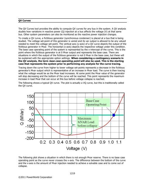
- Page 1248 and 1249: To use the QV Curves tool, select Q
- Page 1250 and 1251: Clicking this button will prompt fo
- Page 1252 and 1253: Step Size Increment between voltage
- Page 1254 and 1255: QV Curves Options: Solution These o
- Page 1256 and 1257: QV Curves Options: Contingencies Th
- Page 1258 and 1259: QV Curves Options: Output These opt
- Page 1260 and 1261: If curves are not plotted at they a
- Page 1262 and 1263: PV/QV Quantities to Track Specifica
- Page 1264 and 1265: Note: all branches (whether transmi
- Page 1266 and 1267: To track the limits of any of these
- Page 1268 and 1269: QV Curves Results: Listing The List
- Page 1270 and 1271: PV/QV Curves Results: Plot Plotting
- Page 1272 and 1273: PV/QV Curves Results: Track Limits
- Page 1274 and 1275: Close Click this button to close th
- Page 1276 and 1277: OPF Objective Function The objectiv
- Page 1278 and 1279: OPF Equality Constraints Area MW In
- Page 1280 and 1281: Each branch that is active for enfo
- Page 1282 and 1283: OPF Unenforceable Constraints The g
- Page 1284 and 1285: OPF Primal LP Go to the Add Ons rib
- Page 1286 and 1287: OPF Options and Results The OPF Opt
- Page 1288 and 1289: shifting transformer, and to avoid
- Page 1290 and 1291: CA (contingency analysis) and SCOPF
- Page 1292 and 1293: done if the Generator Cost Modeling
- Page 1294 and 1295: OPF Options: Advanced Options Detec
- Page 1296 and 1297:
©2011 PowerWorld Corporation Line
- Page 1298 and 1299:
OPF Options: All LP Variables The O
- Page 1300 and 1301:
OPF Options: LP Basis Matrix The OP
- Page 1302 and 1303:
OPF Options: Bus MVAR Marginal Pric
- Page 1304 and 1305:
OPF Options: Inverse of LP Basis Th
- Page 1306 and 1307:
OPF Area Records Displays OPF speci
- Page 1308 and 1309:
OPF Bus Records Displays OPF specif
- Page 1310 and 1311:
"No" - Generator is NOT available a
- Page 1312 and 1313:
OPF Interface Records Displays OPF
- Page 1314 and 1315:
OPF Line/Transformer Records Displa
- Page 1316 and 1317:
OPF Load Records Displays OPF speci
- Page 1318 and 1319:
OPF Super Area Records Displays OPF
- Page 1320 and 1321:
OPF Controls The following classes
- Page 1322 and 1323:
OPF Example - Introduction As a sim
- Page 1324 and 1325:
B7OPF Case Solved using LP OPF with
- Page 1326 and 1327:
OPF Example - Super Areas To jointl
- Page 1328 and 1329:
OPF Example - Enforcing Line MVA Co
- Page 1330 and 1331:
Security Constrained Optimal Power
- Page 1332 and 1333:
SCOPF Dialog The SCOPF dialog allow
- Page 1334 and 1335:
SCOPF Results The Results page of t
- Page 1336 and 1337:
SCOPF Equality Constraints The SCOP
- Page 1338 and 1339:
Each branch that is active for enfo
- Page 1340 and 1341:
the SCOPF does not resolve the cont
- Page 1342 and 1343:
SCOPF CTG Violations The contingenc
- Page 1344 and 1345:
SCOPF LP Solution Details The LP So
- Page 1346 and 1347:
At Breakpoint Yes, if the LP variab
- Page 1348 and 1349:
SCOPF LP Basis Matrix The LP Basis
- Page 1350 and 1351:
SCOPF Bus Marginal Controls This di
- Page 1352 and 1353:
©2011 PowerWorld Corporation B7SCO
- Page 1354 and 1355:
SCOPF Example: Marginal Prices Usin
- Page 1356 and 1357:
Optimal Power Flow Reserves Overvie
- Page 1358 and 1359:
OPF Reserves Controls Generators ca
- Page 1360 and 1361:
OPF Reserves Constraints Reserve co
- Page 1362 and 1363:
OPF Reserves Objective Function The
- Page 1364 and 1365:
OPF Reserves Case Information Displ
- Page 1366 and 1367:
Then, let us set up the following r
- Page 1368 and 1369:
It should be mentioned that OPF Res
- Page 1370 and 1371:
Available Transfer Capability Dialo
- Page 1372 and 1373:
ATC Dialog Options: Common Options
- Page 1374 and 1375:
Contingency elements have an associ
- Page 1376 and 1377:
ATC Dialog Common Options: Transfer
- Page 1378 and 1379:
Line D contains transfer limiter fo
- Page 1380 and 1381:
Linearize Makeup Power Calculation
- Page 1382 and 1383:
Because the goal is to stress the s
- Page 1384 and 1385:
ATC Extra Monitors Dialog Simulator
- Page 1386 and 1387:
ATC Dialog: Result The Result page
- Page 1388 and 1389:
Note: This does not immediately abo
- Page 1390 and 1391:
See Scenarios page for more informa
- Page 1392 and 1393:
Multiple Scenario ATC Dialog: Scena
- Page 1394 and 1395:
injection change exceeds a certain
- Page 1396 and 1397:
One axis has heading labels G0, G1,
- Page 1398 and 1399:
Multiple Scenario ATC Dialog: Combi
- Page 1400 and 1401:
The Branch Limiters tab only shows
- Page 1402 and 1403:
This is the OTDF (or PTDF if the Li
- Page 1404 and 1405:
ATC Analysis Methods: Single Linear
- Page 1406 and 1407:
stepsize so as much as possible of
- Page 1408 and 1409:
ATC Analysis Methods: Iterated Line
- Page 1410 and 1411:
o This step removes the contingency
- Page 1412 and 1413:
Simulator Automation Server (SimAut
- Page 1414 and 1415:
Including Simulator Automation Serv
- Page 1416 and 1417:
Microsoft Visual C++ Declare a var
- Page 1418 and 1419:
Getting Data from the Simulator Aut
- Page 1420 and 1421:
ChangeParameters Function The Chang
- Page 1422 and 1423:
ChangeParametersSingleElement Sampl
- Page 1424 and 1425:
ChangeParametersMultipleElement Fun
- Page 1426 and 1427:
Output = SimAuto.ChangeParametersMu
- Page 1428 and 1429:
ChangeParametersMultipleElementFlat
- Page 1430 and 1431:
CloseCase Function The CloseCase fu
- Page 1432 and 1433:
GetFieldList Function The GetFieldL
- Page 1434 and 1435:
GetParametersSingleElement Function
- Page 1436 and 1437:
GetParametersSingleElement Function
- Page 1438 and 1439:
GetParametersSingleElement Function
- Page 1440 and 1441:
GetParametersSingleElement Function
- Page 1442 and 1443:
GetParametersMultipleElement Functi
- Page 1444 and 1445:
GetParametersMultipleElement Sample
- Page 1446 and 1447:
disp(fieldarray) disp(busesparam) e
- Page 1448 and 1449:
Dim lowobj, highobj As Integer lowo
- Page 1450 and 1451:
GetParameters Function This functio
- Page 1452 and 1453:
As you can see, to access the first
- Page 1454 and 1455:
end; end; end; ©2011 PowerWorld Co
- Page 1456 and 1457:
num2str(devicelist2(counter)) ' ' .
- Page 1458 and 1459:
DisplayMessage "Number of Key Field
- Page 1460 and 1461:
ListOfDevicesFlatOutput Function Th
- Page 1462 and 1463:
LoadState Function: Sample Code Mic
- Page 1464 and 1465:
OpenCase Function: Sample Code Borl
- Page 1466 and 1467:
ProcessAuxFile Function: Sample Cod
- Page 1468 and 1469:
RunScriptCommand Function: Sample C
- Page 1470 and 1471:
SaveCase Function: Sample Code Micr
- Page 1472 and 1473:
SaveState Function: Sample Code Mic
- Page 1474 and 1475:
SendToExcel Function: Sample Code M
- Page 1476 and 1477:
©2011 PowerWorld Corporation 1448
- Page 1478 and 1479:
©2011 PowerWorld Corporation 1450
- Page 1480 and 1481:
%Delete (close) the COM object. del
- Page 1482 and 1483:
WriteAuxFile Function: Sample Code
- Page 1484 and 1485:
Simulator Automation Server Propert
- Page 1486 and 1487:
ExcelApp Property: Sample Code Micr
- Page 1488 and 1489:
CurrentDir Property: Sample Code Mi
- Page 1490 and 1491:
ProcessID Property: Sample Code Mic
- Page 1492 and 1493:
PowerWorld Object Variables The abi
- Page 1494 and 1495:
Installing Simulator Automation Ser
- Page 1496 and 1497:
Connecting to Simulator Automation
- Page 1498 and 1499:
Simulator Automation Server Propert
- Page 1500 and 1501:
Simulator Automation Server Functio
- Page 1502 and 1503:
CloseCase Function (version 9) The
- Page 1504 and 1505:
ListOfDevices Function (version 9)
- Page 1506 and 1507:
OpenCase Function (version 9) The O
- Page 1508 and 1509:
RunScriptCommand Function (version
- Page 1510 and 1511:
SendToExcel Function (version 9) Th
- Page 1512 and 1513:
PowerWorld Object Variables (Versio
- Page 1514 and 1515:
Integrated Topology Processing Over
- Page 1516 and 1517:
Integrated Topology Processing: Ful
- Page 1518 and 1519:
Integrated Topology Processing: Sup
- Page 1520 and 1521:
Integrated Topology Processing: Con
- Page 1522 and 1523:
Integrated Topology Processing Cons
- Page 1524 and 1525:
Integrated Topology Processing: Con
- Page 1526 and 1527:
Integrated Topology Processing Dial
- Page 1528 and 1529:
Integrated Topology Processing: Pow
- Page 1530 and 1531:
Integrated Topology Processing: Con
- Page 1532 and 1533:
Contingency Element: Open Breakers
- Page 1534 and 1535:
Integrated Topology Processing: Inc
- Page 1536 and 1537:
Integrated Topology Processing: Sav
- Page 1538 and 1539:
Integrated Topology Processing: Sav
- Page 1540 and 1541:
Provides the mapping used when solv
- Page 1542 and 1543:
Device Derived Status Differences e
- Page 1544 and 1545:
In this last example, additional br
- Page 1546 and 1547:
Transient Stability Overview The Tr
- Page 1548 and 1549:
Governor Response Limits There is a
- Page 1550 and 1551:
©2011 PowerWorld Corporation 1522
- Page 1552 and 1553:
The WT1G model is the GE DYD repres
- Page 1554 and 1555:
Transient Stability Overview: Loads
- Page 1556 and 1557:
Transient Contour Toolbar The Trans
- Page 1558 and 1559:
Transient Stability Numerical Integ
- Page 1560 and 1561:
Transient Stability Overview: PlayI
- Page 1562 and 1563:
Transient Stability: Model Data Man
- Page 1564 and 1565:
When clicking this button, the Bloc
- Page 1566 and 1567:
Transient Stability Case Info Menu
- Page 1568 and 1569:
Choose the appropriate option to sa
- Page 1570 and 1571:
All On the listing which shows all
- Page 1572 and 1573:
Transient Stability Data: Block Dia
- Page 1574 and 1575:
model suite. The CAPRELAY model can
- Page 1576 and 1577:
Transient Limit Monitors States/Man
- Page 1578 and 1579:
Transient Stability Analysis: Simul
- Page 1580 and 1581:
Transient Stability Contingency Ele
- Page 1582 and 1583:
OK Fault Type - Balanced 3 Phase, S
- Page 1584 and 1585:
Transient Stability Analysis Option
- Page 1586 and 1587:
When this option is checked, an est
- Page 1588 and 1589:
higher than nominal frequency, then
- Page 1590 and 1591:
Transient Stability Dialog Options:
- Page 1592 and 1593:
Transient Stability Dialog Options:
- Page 1594 and 1595:
©2011 PowerWorld Corporation 1566
- Page 1596 and 1597:
Set All NO Click the Set All NO but
- Page 1598 and 1599:
Make Plot This button is enabled wh
- Page 1600 and 1601:
A list of objects types for which t
- Page 1602 and 1603:
A more complicated example consisti
- Page 1604 and 1605:
©2011 PowerWorld Corporation 1576
- Page 1606 and 1607:
Click the Add Plot button found on
- Page 1608 and 1609:
Axis group selected - axis groups w
- Page 1610 and 1611:
Transient Stability Analysis Plot D
- Page 1612 and 1613:
Transient Stability Analysis Plot D
- Page 1614 and 1615:
Transient Stability Analysis Plot D
- Page 1616 and 1617:
Transient Stability Analysis Plot D
- Page 1618 and 1619:
Transient Stability Analysis Plot D
- Page 1620 and 1621:
Transient Stability Analysis Plot D
- Page 1622 and 1623:
Solid, Dashed, Dot, Dash Dot, and D
- Page 1624 and 1625:
Provides access to export images, b
- Page 1626 and 1627:
Transient Stability : Defining Tran
- Page 1628 and 1629:
toolbar and then choosing the appro
- Page 1630 and 1631:
value occurs. Note that point B may
- Page 1632 and 1633:
Analysis time at which the maximum
- Page 1634 and 1635:
Transient Stability Analysis: State
- Page 1636 and 1637:
Transient Stability Analysis: Valid
- Page 1638 and 1639:
if Xl > Xqpp then Xl = 0.8*Xqpp if
- Page 1640 and 1641:
In addition to getting the eigenval
- Page 1642 and 1643:
plot will be drawn. When creating a
- Page 1644 and 1645:
Distributed Computing Add-Ons The D
- Page 1646 and 1647:
Tutorial: Creating a New Case Page
- Page 1648 and 1649:
The Bus Number field automatically
- Page 1650 and 1651:
Click OK on the Generator Option Di
- Page 1652 and 1653:
Tutorial: Entering a Second Bus wit
- Page 1654 and 1655:
©2011 PowerWorld Corporation 1626
- Page 1656 and 1657:
The Series Resistance, Series React
- Page 1658 and 1659:
©2011 PowerWorld Corporation 1630
- Page 1660 and 1661:
©2011 PowerWorld Corporation 1632
- Page 1662 and 1663:
atio of nominal voltages between th
- Page 1664 and 1665:
Tutorial: Inserting a Switched Shun
- Page 1666 and 1667:
Tutorial: Inserting Text, Bus and L
- Page 1668 and 1669:
The parameter and position are disp
- Page 1670 and 1671:
Tutorial: Solving the Case Page 12
- Page 1672 and 1673:
Tutorial: Adding a New Area Page 13
- Page 1674 and 1675:
Change the Area Name to ‘One’ a
- Page 1676 and 1677:
Tutorial: Loading an Existing Power
- Page 1678 and 1679:
Tutorial: Solving the Case Page 4 o
- Page 1680 and 1681:
Tutorial: Entering a Bus Page 6 of
- Page 1682 and 1683:
Panning and Zooming Page 8 of 15 Tw
- Page 1684 and 1685:
Tutorial: Simulating the Case Page
- Page 1686 and 1687:
Oneline Local Menu Page 12 of 15 Se
- Page 1688 and 1689:
Limit Violations Page 14 of 15 You
- Page 1690 and 1691:
Tutorial: Solving an OPF Page 1 of
- Page 1692 and 1693:
Tutorial: OPF Line Limit Enforcemen
- Page 1694 and 1695:
Tutorial: OPF Marginal Cost of Enfo
- Page 1696 and 1697:
B3LP Solved with Unenforceable Cons
- Page 1698 and 1699:
Area Buses, 428 Area Gens, 429 Area
- Page 1700 and 1701:
ChangeParametersMultipleElement Sam
- Page 1702 and 1703:
DC Transmission Line Options, 350 D
- Page 1704 and 1705:
General, 489, 622, 654 General Scri
- Page 1706 and 1707:
Jacobian, 97, 284 Key Field, 664 Ke
- Page 1708 and 1709:
Mouse Wheel Zooming, 828 Movie Make
- Page 1710 and 1711:
Palettes, 776, 777 ©2011 PowerWorl
- Page 1712 and 1713:
Quick Access Toolbar, 29 Tools, 57
- Page 1714 and 1715:
Sensitivities, 986, 991, 996, 997,
- Page 1716 and 1717:
Schedule Subscription Dialog, 1152
- Page 1718:
X Grid Spacing, 798 XF, 255 x-y, 87