- Page 1:
Preparatory Notes for ASNT NDT Leve
- Page 6 and 7:
Numerical Prefix • Micro - (µ) a
- Page 8 and 9:
Contents: 1. ASNT Level III Exam To
- Page 10 and 11:
4. Interpretation/Evaluations • E
- Page 12 and 13:
UT - Ultrasonic Testing Length: 4 h
- Page 14 and 15:
3. Techniques/Calibrations •Conta
- Page 16 and 17:
ASME V Article Numbers: Gen Article
- Page 18:
Other Reading • http://techcorr.c
- Page 21 and 22:
Content: Section 1: Introduction 1.
- Page 23 and 24:
Content: Section 3: Equipment & Tra
- Page 25 and 26:
Content: Section 4: Calibration Met
- Page 27 and 28:
Content: Section 6: Selected Applic
- Page 29 and 30:
Section 1: Introduction
- Page 31 and 32:
1.1: Basic Principles of Ultrasonic
- Page 33 and 34:
In ultrasonic testing, the reflecte
- Page 35 and 36:
Basics of Ultrasonic Test- Contact
- Page 37 and 38:
Basics of Ultrasonic Test- A-Scan
- Page 39 and 40:
Source-2: The advantages of ultraso
- Page 41 and 42:
• Operation is electronic, which
- Page 43 and 44:
1.3: Limitations (Disadvantages) As
- Page 46 and 47:
Content: Section 2: Physics of Ultr
- Page 48 and 49:
Ultrasonic Formula
- Page 50:
Parameters of Ultrasonic Waves
- Page 53 and 54:
Acoustic Spectrum
- Page 55 and 56:
Acoustic Spectrum
- Page 57 and 58:
Acoustic Wave - Node and Anti-Node
- Page 59 and 60:
Q151 A point, line or surface of a
- Page 61 and 62:
2.2.2 Propagation & Polarization Ve
- Page 63 and 64:
Longitudinal and shear waves- Defin
- Page 65 and 66:
Longitudinal and shear waves
- Page 67 and 68:
In longitudinal waves, the oscillat
- Page 69:
Longitudinal Wave
- Page 72 and 73:
Shear waves vibrate particles at ri
- Page 74:
In the transverse or shear wave, th
- Page 77 and 78:
2.2.5 Rayleigh Characteristics Rayl
- Page 79 and 80:
Rayleigh waves
- Page 81 and 82:
Surface (or Rayleigh) waves travel
- Page 83 and 84:
The major axis of the ellipse is pe
- Page 85 and 86:
Surface wave or Rayleigh wave are f
- Page 87 and 88:
Surface wave - Following Contour Su
- Page 89 and 90:
Rayleigh Wave http://web.ics.purdue
- Page 91 and 92:
Love Wave
- Page 93 and 94:
At this depth, wave energy is about
- Page 95 and 96:
Q: Which of the following modes of
- Page 97 and 98:
Since the 1990s, the understanding
- Page 99 and 100:
Plate or Lamb waves are the most co
- Page 101 and 102:
Plate wave or Lamb wave are formed
- Page 103 and 104:
When guided in layers they are refe
- Page 105 and 106:
Symmetrical = extensional mode Asym
- Page 107 and 108:
Other Reading: Lamb Wave Lamb waves
- Page 109 and 110:
Fig. 4 Diagram of the basic pattern
- Page 111 and 112:
2.2.7 Dispersive Wave: Wave modes s
- Page 113 and 114:
Plate or Lamb waves are generated a
- Page 115 and 116:
2.3: Sound Propagation in Elastic M
- Page 117 and 118:
Spring model- A mass on a spring ha
- Page 119 and 120:
Elastic Model
- Page 121 and 122:
Elastic Model / Longitudinal Wave
- Page 123 and 124:
Elastic Model / Shear Wave
- Page 125 and 126:
Since the mass m and the spring con
- Page 127 and 128:
Elastic constant → spring constan
- Page 129 and 130:
Q163 Acoustic velocity of materials
- Page 131 and 132:
When calculating the velocity of a
- Page 133 and 134:
It must also be mentioned that the
- Page 135 and 136:
Longitudinal Wave Velocity: V L The
- Page 137 and 138:
2.4: Properties of Acoustic Plane W
- Page 139 and 140:
http://www.ndt-ed.org/EducationReso
- Page 141 and 142:
Java don’t work? Uninstalled →
- Page 143 and 144:
Java don’t work? http://jingyan.b
- Page 145 and 146:
Java don’t work? http://jingyan.b
- Page 147 and 148:
The velocities sound waves The velo
- Page 149 and 150:
2.5: Wavelength and Defect Detectio
- Page 151 and 152:
Keywords: • Discontinuity must be
- Page 153 and 154:
Keywords: • Coarse grains →Lowe
- Page 155 and 156:
Coarse grains →Lower frequency to
- Page 157 and 158:
Keywords: • Higher the frequency,
- Page 159 and 160:
2.5.3 Further Reading Detectability
- Page 162 and 163:
Determining cross sectional area us
- Page 164 and 165:
“Sonic pulse volume” and S/N (d
- Page 166 and 167:
2.6: Attenuation of Sound Waves 2.6
- Page 168 and 169:
Absorption: Sound attenuations are
- Page 170 and 171:
Anisotropic Columnar Grains with di
- Page 172 and 173:
The amplitude change of a decaying
- Page 174 and 175:
Attenuation is generally proportion
- Page 176 and 177:
Amplitude at distance Z where: Wher
- Page 178:
2.6.2 Factors Affecting Attenuation
- Page 181 and 182:
2.6.4 Further Reading on Attenuatio
- Page 183 and 184:
Q168: Heat conduction, viscous fric
- Page 185 and 186:
2.7: Acoustic Impedance Acoustic im
- Page 187 and 188:
Sound travels through materials und
- Page 189 and 190:
Reflection/Transmission Energy as a
- Page 191 and 192:
Q2.8: The acoustic impedance of mat
- Page 193 and 194:
When the acoustic impedances of the
- Page 195 and 196:
Reflection Coefficient:
- Page 197 and 198:
Using the above applet, note that t
- Page 199 and 200:
Incident Wave other than Normal? -
- Page 201 and 202:
Q: The figure above shown the parti
- Page 203 and 204:
For example: The dB loss on transmi
- Page 205 and 206:
Q6: For an ultrasonic beam with nor
- Page 207 and 208:
Refraction and Snell's Law When an
- Page 210 and 211:
Refraction takes place at an interf
- Page 212:
Snell's Law describes the relations
- Page 216 and 217:
Snell Law http://www.ndt-ed.org/Edu
- Page 218 and 219:
When a longitudinal wave moves from
- Page 220 and 221:
Refraction and mode conversion occu
- Page 222 and 223:
For example, calculate the first cr
- Page 224 and 225:
Snell Law: 1 st / 2 nd Critical Ang
- Page 226 and 227:
Q. Both longitudinal and shear wave
- Page 234 and 235:
Typical angle beam assemblies make
- Page 236 and 237:
Depth & Skip
- Page 238 and 239:
Second Critical Angle The second cr
- Page 240 and 241:
2.10: Mode Conversion When sound tr
- Page 242 and 243:
In the previous section, it was poi
- Page 244 and 245:
Snell's Law
- Page 246 and 247:
Reflections
- Page 248 and 249:
V S1 V S2
- Page 250 and 251:
Snell Law- 1 st & 2 nd Critical Ang
- Page 252 and 253:
Transverse wave can be introduced i
- Page 254 and 255:
Calculate the offset for following
- Page 256 and 257:
Refraction and mode conversion at n
- Page 258 and 259:
Refraction and mode conversion at n
- Page 260 and 261:
Q1. From the above figures, if the
- Page 262 and 263:
Q: On Calculation: Incident angle=
- Page 264 and 265:
Q1. If you were requested to design
- Page 266 and 267:
2.11: Signal-to-Noise Ratio In a pr
- Page 268 and 269:
The following formula relates some
- Page 270 and 271:
Rather than go into the details of
- Page 273 and 274:
Determining cross sectional area us
- Page 275 and 276:
“Sonic pulse volume” and S/N (d
- Page 277 and 278:
Pulse Length
- Page 279 and 280:
2.12: The Sound Fields 2.12.1 Wave
- Page 281 and 282:
When waves interact, they superimpo
- Page 283 and 284:
UT Transducer http://www.fhwa.dot.g
- Page 285 and 286:
UT Transducer
- Page 287 and 288:
Wave Interaction Complete in-phase
- Page 289 and 290:
With an ultrasonic transducer, the
- Page 291 and 292:
29. It is possible for a discontinu
- Page 293 and 294:
2.12.2 Variations in sound intensit
- Page 295 and 296:
The sound wave exit from a transduc
- Page 297 and 298:
The Near Field (Fresnel) and the Fa
- Page 299 and 300:
Amplitude ← Near Field Effect: Be
- Page 301 and 302:
Near field (near zone) or Fresnel z
- Page 303 and 304:
Near/ Far Fields http://miac.unibas
- Page 305 and 306:
where α is the radius of the trans
- Page 307 and 308:
The curvature and the area over whi
- Page 309 and 310:
Fresnel & Fraunhofer Zone
- Page 311 and 312:
Fresnel & Fraunhofer Zone http://st
- Page 313 and 314:
Q4: A transducer has a near field i
- Page 315 and 316:
2.12.4 Dead Zone In ultrasonic test
- Page 317 and 318:
Dead Zone -The initial pulse is a t
- Page 319 and 320:
Dead Zone Illustration http://www.n
- Page 321 and 322:
Q: On an A-scan display, the “dea
- Page 323 and 324:
2.13: Inverse Square Rule/ Inverse
- Page 325 and 326:
Small Reflector, a reflector smalle
- Page 329 and 330:
2.14: Resonance Another form wave i
- Page 331 and 332:
Thickness of Crystal at Fundamental
- Page 333 and 334:
Resonance UT Testing- The diagram b
- Page 335 and 336:
From the natural frequencies it is
- Page 337 and 338:
Q: The formula used to determine th
- Page 339 and 340:
2.15 Measurement of Sound
- Page 341 and 342:
Ultrasonic Formula - Signal Amplitu
- Page 343 and 344:
where: delta X is the difference in
- Page 345 and 346:
From this table it can be seen that
- Page 347 and 348:
However, the power or intensity of
- Page 349 and 350:
Revising the table to reflect the r
- Page 351 and 352:
Sound Levels- Relative dB
- Page 353 and 354:
“Absolute" Sound Levels Sound pre
- Page 356 and 357:
dB meter 97.3dB against standards s
- Page 358 and 359:
Exercise: Find the absolute sound l
- Page 360 and 361:
Practice: dB
- Page 362 and 363:
Example Calculation 2 If the intens
- Page 364 and 365:
What is the absolute rock concert s
- Page 366 and 367:
Practice Makes Perfect 28. An advan
- Page 368 and 369:
学 习 总 是 开 心 事
- Page 370 and 371:
学 习 总 是 开 心 事
- Page 372 and 373:
学 习 总 是 开 心 事
- Page 374 and 375:
学 习 总 是 开 心 事
- Page 376 and 377:
学 习 总 是 开 心 事
- Page 379 and 380:
Typical sound velocities
- Page 381 and 382:
Content: Section 3: Equipment & Tra
- Page 383 and 384:
3.1: Piezoelectric Transducers The
- Page 385 and 386:
Pulse width (PW) - the time duratio
- Page 387 and 388:
Piezoelectric Properties The conver
- Page 389 and 390:
Fig. 5.10: Basic design of a single
- Page 391 and 392:
Piezoelectric crystals http://www.n
- Page 393 and 394:
Piezoelectric crystals
- Page 395 and 396:
Piezoelectric crystals
- Page 397 and 398:
The active element of most acoustic
- Page 399 and 400:
The fundamental frequency of the tr
- Page 401 and 402:
At Interface: Reflection & Transmit
- Page 403 and 404:
At Interface: Reflection & Transmit
- Page 405 and 406:
Piezoelectric crystals
- Page 407 and 408:
Piezoelectric crystals
- Page 409 and 410:
Piezoelectric crystals
- Page 411 and 412:
■ Quartz is a Silicon Oxide (SiO
- Page 413 and 414:
SiO3-Silicon Quartz
- Page 415 and 416:
Lithium Sulphate LiSO 4 硫 酸 锂
- Page 417 and 418:
■ Barium Titanate (BaTiO 3 ) are
- Page 419 and 420:
BaTiO 3
- Page 421 and 422:
Fig. 3: Comparison between PZT (lef
- Page 423 and 424:
■ Lead Zirconate Titanate (PBZrO
- Page 425 and 426:
350°C is also goof for:
- Page 427 and 428:
350°C is also goof for:
- Page 429 and 430:
Lead zirconium Titanate is an inter
- Page 431:
http://www.ndt.net/article/platte2/
- Page 434 and 435:
Ceramic Transducer
- Page 436 and 437:
Q68: Which of the following transdu
- Page 438 and 439:
Q73: Which of the following is the
- Page 440 and 441:
Transducer
- Page 442 and 443:
3.2.1 Transducer Cut-Out A cut away
- Page 444 and 445:
Transducer
- Page 446 and 447:
Transducer: Angle Beam
- Page 448 and 449:
3.2.2 The Active Element (Crystal)
- Page 450 and 451:
Matching Layer: Immersion & Delay T
- Page 452 and 453:
Note on Backing: The backing materi
- Page 454 and 455:
Matching Layer (Wear Plate) For imm
- Page 456 and 457:
Transducers
- Page 458 and 459:
3.2.6 Transducer Efficiency, Bandwi
- Page 460 and 461:
2 λ 50% Amplitude or 6dB line. 2
- Page 463 and 464:
3.2.6.2 Transducer Damping It is al
- Page 465 and 466:
Transducer (Backing) Damping: • H
- Page 467 and 468:
Transducer Damping
- Page 469 and 470:
Transducer Damping at -20dB
- Page 471 and 472:
Transducer Damping
- Page 473 and 474:
Wave form Duration at -10dB
- Page 475 and 476:
Transducer Damping- High Damping (X
- Page 477 and 478:
3.2.6.3 Bandwidth: It is also impor
- Page 479 and 480:
The central frequency will also def
- Page 481 and 482:
Bandwidth (BW) - the difference bet
- Page 483 and 484:
Transducers are constructed to with
- Page 485 and 486:
Instrumentation Filtered Band Width
- Page 487 and 488:
Q8: Receiver noise must often be fi
- Page 489 and 490:
Q48: The approximate bandwidth of t
- Page 491:
Since the ultrasound originates fro
- Page 494 and 495:
Near Field
- Page 496 and 497:
Angular characteristics: Lines of e
- Page 498 and 499:
Angular characteristics: Sound-pres
- Page 500 and 501:
For a piston source transducer of r
- Page 502 and 503:
Spherical or cylindrical focusing c
- Page 504 and 505:
Probe Dimension & Spread angle 探
- Page 506 and 507:
Probe dimension & Z f , , Ɵ 探
- Page 508 and 509:
3.4: Transducer Beam Spread As disc
- Page 510 and 511:
As shown in the applet below, beam
- Page 513 and 514:
Beam angle is an important consider
- Page 515 and 516:
3.5: Transducer Types Ultrasonic tr
- Page 517 and 518:
Contact Transducers
- Page 519 and 520:
Contact Transducer http://www.olymp
- Page 521 and 522:
3.5.2 Immersion transducers In imme
- Page 523 and 524:
Focusing Ration in water/steel (F=4
- Page 525 and 526:
Focal Length Equation: The focal le
- Page 527 and 528:
Focal Length Variations
- Page 529 and 530:
Cylindrical & Spherical Focused
- Page 531 and 532:
Q79: What type of search unit allow
- Page 533 and 534:
Q78: Which of the following is not
- Page 535 and 536:
For a single crystal probe the leng
- Page 537 and 538:
There are other advantages 1. Doubl
- Page 539 and 540:
Advantages: Improves near surface r
- Page 541 and 542:
Duo Elements Transducer Transmittin
- Page 543 and 544:
3.5.4 Delay line transducers provid
- Page 545 and 546:
Other Reading (Olympus): Delay Line
- Page 547:
Delay lined Transducer
- Page 550 and 551:
Probe Delay with TR-Probe
- Page 552 and 553:
Probe Delay
- Page 554 and 555:
Delay Line UT 1 Lab 8 www.youtube.c
- Page 556 and 557:
Angle Beam Transducers- Angle beam
- Page 558 and 559:
Angle Beam Transducers- Angle beam
- Page 560 and 561:
Angle Beam Transducers- Angle beam
- Page 562 and 563:
Angle Beam Transducers- Angle beam
- Page 564 and 565:
Angle Beam Transducers- Angle beam
- Page 566 and 567:
Angle Beam Transducers ϴ 1L ϴ 2L
- Page 568 and 569:
Angle Beam Transducers- Mode Conver
- Page 570 and 571:
Angle Beam Transducers- Common Term
- Page 572 and 573:
Angle Beam Transducer http://www.ol
- Page 574 and 575:
Application of Normal incidence she
- Page 576 and 577:
Normal incidence shear wave transdu
- Page 578 and 579:
Q: To evaluate and accurately locat
- Page 580 and 581:
Q: A special scanning device with t
- Page 582 and 583:
3.6: Transducer Testing Some transd
- Page 584 and 585:
TRANSDUCER EXCITATION As a general
- Page 586 and 587:
Square Wave Spiked Pulser: (negativ
- Page 588 and 589:
UT Flaw Detector - Olympus EPOCH 60
- Page 590 and 591:
Effects of Probe Frequencies: 1. Hi
- Page 594 and 595:
As noted in the ASTM E1065 Standard
- Page 596 and 597:
Relative Pulse-Echo Sensitivity--Th
- Page 598 and 599:
Sound Field Measurements--The objec
- Page 600 and 601:
There is ongoing research to develo
- Page 602 and 603:
3.8: Couplants A couplant is a mate
- Page 604 and 605:
Immersion Method - Water as a coupl
- Page 606 and 607:
Squirter Column (bubbler)- Water as
- Page 608 and 609:
Couplant
- Page 610 and 611:
Electromagnetic-acoustic transducer
- Page 612 and 613:
EMAT
- Page 614 and 615:
Electromagnetic acoustic transducer
- Page 616 and 617:
3. Dry Inspection. Since no couplan
- Page 618 and 619:
Applications of EMATs EMAT has been
- Page 620 and 621:
Cross-sectional view of a spiral co
- Page 622 and 623:
Cross-sectional view of a tangentia
- Page 624 and 625:
EMATS The bulk-shear-wave EMAT cons
- Page 626 and 627:
Cross-sectional view of a periodic
- Page 628 and 629:
3.10: Pulser-Receivers Ultrasonic p
- Page 630 and 631:
Transducer Cut-out
- Page 632 and 633:
Pulse Length: BS4331 Pt2. N= Pulse
- Page 634:
Pulse Length: A long pulse length m
- Page 637 and 638:
Pulse Length
- Page 639 and 640:
Pulse Length
- Page 641 and 642:
Pulse-Length and Wave form Quality
- Page 643 and 644:
Pulse Length- x axis time domain Qu
- Page 645 and 646:
Pulse-echo mode of operation, wideb
- Page 647 and 648:
Sensitivity in pulse-echo mode of o
- Page 649 and 650:
Damping: Shock wave transducer and
- Page 651 and 652:
The pulser-receiver is also used in
- Page 653 and 654:
Transducers of the kind most common
- Page 655 and 656:
Bandwidth - Typical transducers for
- Page 657 and 658:
In fact, the actual beam profile is
- Page 659 and 660:
Attenuation - As it travels through
- Page 661 and 662:
3.11: Tone Burst Generators In Rese
- Page 663 and 664:
Tone burst generators http://www.se
- Page 665 and 666:
Section of biphase modulated spread
- Page 667 and 668:
3.13: Electrical Impedance Matching
- Page 669 and 670:
Cable Electrical Characteristics Th
- Page 671 and 672:
Capacitance in a cable is usually m
- Page 673 and 674:
Quality Factor “Q”
- Page 675 and 676:
3.15: Data Presentation Ultrasonic
- Page 677 and 678:
Data Presentation:
- Page 679 and 680:
In the A-scan presentation, relativ
- Page 681 and 682:
A-Scan http://static3.olympus-ims.c
- Page 683 and 684:
3.15.2 B-Scan http://static2.olympu
- Page 685 and 686:
B-Scan http://static2.olympus-ims.c
- Page 687 and 688:
It should be noted that a limitatio
- Page 689 and 690:
Q: In a B-scan display, the length
- Page 691 and 692:
C-Scan The (1) relative signal ampl
- Page 694 and 695:
C-Scan / A-Scan
- Page 696 and 697:
C-Scan
- Page 698 and 699:
C-Scan Recording
- Page 700 and 701:
The D scan- The D scan gives a side
- Page 702 and 703:
3.15.5 The Through Transmission Sha
- Page 704 and 705:
Fig. 12.1 Principle of the shadow m
- Page 706 and 707:
3.15.6 Other Presentations
- Page 708 and 709:
3.16.2 Through Transmission Techniq
- Page 711 and 712:
The Through Transmission Shadow Met
- Page 713 and 714:
The Tandem Techniques Phased array:
- Page 715 and 716:
During the set-up of immersion meth
- Page 717 and 718:
3.17 UT Equipment Circuitry & Contr
- Page 719 and 720:
Instrument Circuitry: Time base The
- Page 721 and 722:
Instrument Circuitry: Power Supply.
- Page 723 and 724:
Instrument Circuitry: Signal-condit
- Page 725 and 726:
Instrument Circuitry: Clock The clo
- Page 727 and 728:
Instrument Circuitry: Pulser-Receiv
- Page 729 and 730:
Instrument Control: REJECT Control
- Page 731 and 732:
Instrument Control: GAIN Control Th
- Page 733 and 734:
• A control that varies the level
- Page 735 and 736:
• High-voltage or low-voltage dri
- Page 737 and 738:
3.17.3 Pulse-Echo Instrumentation (
- Page 739:
3. The voltage pulse reaches the tr
- Page 742 and 743:
Typical block diagram of an analog
- Page 744 and 745:
3.17.4 B Scan Block diagram: B-scan
- Page 746 and 747:
Typical B-scan setup, including vid
- Page 748 and 749:
• Third, echoes are indicated by
- Page 750 and 751:
3.17.5 C-scan display C-scan displa
- Page 752 and 753:
System Setup. In a basic C-scan sys
- Page 754 and 755:
Q79: In the pulse echo instrument,
- Page 756 and 757:
Q1: The rate generator in B-scan eq
- Page 758 and 759:
Q129: An A-scan display, which show
- Page 760 and 761:
Q32: On many ultrasonic testing ins
- Page 762 and 763:
123. In a basic pulse echo ultrason
- Page 764 and 765:
3.18 Further Reading on Sub-Section
- Page 766 and 767:
In this picture there is two differ
- Page 768 and 769:
This picture shows how water waves
- Page 770 and 771:
3.18.4 Diffraction
- Page 772 and 773:
Diffraction
- Page 774 and 775:
Diffraction
- Page 776 and 777:
Diffraction
- Page 778 and 779:
This diagram shows an interference.
- Page 780 and 781:
Interference
- Page 782 and 783:
3.19 Questions & Answers
- Page 784 and 785:
Q12: The 1 MHz transducer that shou
- Page 786 and 787:
Q4. Calibration of ultrasonic equip
- Page 788 and 789:
Discussion Topic: Factors affecting
- Page 790:
Experts at Work-Salute!
- Page 794 and 795:
Content: Section 4: Calibration Met
- Page 796 and 797:
Calibrations
- Page 798 and 799:
This section will discuss some of t
- Page 800 and 801:
The IIW Type Calibration Block
- Page 802 and 803:
The IIW Type 2 Calibration Block
- Page 804 and 805:
EN12223:1999 Calibration Block
- Page 806 and 807:
The IIW Calibration Block 1 st Chec
- Page 808:
The IIW Calibration Block 2 nd Chec
- Page 812 and 813:
The IIW Phase Array Calibration Blo
- Page 814 and 815:
The IIW 2 Calibration Block Check f
- Page 816 and 817:
Calibration Blocks- Area Amplitude
- Page 818 and 819:
IIW Blocks- US-1 IIW Type US-1
- Page 820 and 821:
IIW Blocks- IIW Type Mini
- Page 822 and 823:
IIW type blocks are used to calibra
- Page 824 and 825:
A block that closely resembles the
- Page 826 and 827:
DSC AWS Block
- Page 828 and 829:
AWS Shear Wave Distance Calibration
- Page 830 and 831:
The DC AWS Block is a metal path di
- Page 832 and 833:
The RC Block is used to determine t
- Page 834 and 835:
Miniature Resolution Block The mini
- Page 836 and 837:
Distance/Sensitivity (DS) Block The
- Page 838 and 839:
The ASTM basic set of Area/Distance
- Page 840 and 841:
Distance/Area-Amplitude Blocks Dist
- Page 842 and 843:
Area-Amplitude Blocks Area-amplitud
- Page 844 and 845:
Key Words: Distance Amplitude Block
- Page 846 and 847:
Q: A primary purpose of a reference
- Page 848 and 849:
DAC Curve
- Page 850 and 851:
DAC- Distance Amplitude Correction
- Page 853 and 854:
A distance amplitude correction cur
- Page 855 and 856:
DAC Java http://www.ndt-ed.org/Educ
- Page 857 and 858:
Sequence for constructing a DAC cur
- Page 859 and 860:
Back Wall Echo Sweep 2” / Distanc
- Page 861 and 862:
3.) Position the transducer over th
- Page 863 and 864:
5.) To complete the DAC curve conne
- Page 865 and 866:
DAC Curve
- Page 867:
Gain Control for FSH: It should be
- Page 870 and 871:
Alta Vista UT Calibration DAC Curve
- Page 872 and 873:
Exit Point A2 Block
- Page 874 and 875:
Q16: Notches are frequently used as
- Page 876 and 877:
Probe Angles- A2 Block
- Page 878 and 879:
4.2.4: Calibration of shear waves f
- Page 880 and 881:
1 st Echo from circular Section
- Page 882 and 883:
Calibration of shear waves for rang
- Page 884 and 885:
25 mm radius from V2 Block
- Page 886 and 887:
100 mm radius from K2 Block
- Page 888 and 889:
Shear Wave Distance Calibration IIW
- Page 890 and 891:
4.2.5: Dead Zone Determine the dead
- Page 892 and 893:
4.2.6: 20 dB Profile- A5 Block
- Page 894 and 895:
20 dB Profile Probe Beam Sound Pres
- Page 896 and 897:
Example: 0 degree Probe Calibration
- Page 898 and 899:
TRANSFER & ATTENUATION CORRECTION:
- Page 900 and 901:
4.2.8: Linearity Checks (Time Base
- Page 902:
Tolerance Unless otherwise specifie
- Page 908 and 909:
4.2.8.2: Linearity of Equipment Gai
- Page 912:
5.2.8.3-1: Linearity of vertical di
- Page 915 and 916:
4.2.8.3-2: Linearity of vertical di
- Page 918 and 919:
4.2.9: Time Correction Gain (TCG) P
- Page 920 and 921:
Q29: Test sensitivity correction fo
- Page 922 and 923:
Convex surfaces work to defocus the
- Page 924 and 925:
convex surfaces work to defocus the
- Page 926 and 927:
Q: In an immersion method, the inci
- Page 928 and 929:
A curvature correction curve can be
- Page 930 and 931:
The plot to the right shows an exam
- Page 932 and 933:
A table of correction values and th
- Page 934 and 935:
Curvature Correction
- Page 936 and 937:
An important source of practice cod
- Page 938 and 939:
Spherical reflectors are often used
- Page 940 and 941:
4.5: Questions & Answers Exercises
- Page 942 and 943:
Q6: The Notches are frequently used
- Page 944 and 945:
Birring NDT Series, UT of Welds Par
- Page 950 and 951:
Section 5: Measurement Techniques
- Page 952 and 953:
Expert at works
- Page 954 and 955:
d 1 = v½t d 2 = v½t = d 1 +d 2 2v
- Page 956 and 957:
A Scan http://www.ndt-ed.org/Educat
- Page 958 and 959:
In thickness gauging, ultrasonic te
- Page 960 and 961:
A-Scan http://www.ndt-ed.org/Educat
- Page 963 and 964:
A-Scan http://www.ndt-ed.org/Educat
- Page 965 and 966:
Flaw Location and Echo Display
- Page 967 and 968:
Flaw Location and Echo Display
- Page 969 and 970:
Flaw Location and Echo Display
- Page 971 and 972:
Near Surface Detectability with Ang
- Page 973 and 974:
Flaw Location with Angle Beam Trans
- Page 975 and 976:
Flaw Location with Angle Beam Trans
- Page 977 and 978:
Why angle beam assemblies are used
- Page 979 and 980:
http://www.olympus-ims.com/en/appli
- Page 981 and 982:
Sound energy that is transmitted fr
- Page 983 and 984:
Selecting the right angle beam asse
- Page 985 and 986:
The IIW recommends the use of a con
- Page 987 and 988:
High temperature wedges Standard an
- Page 989 and 990:
5.3: Reflector Sizing There are man
- Page 991 and 992:
Crack height (a) is a function of t
- Page 993 and 994:
5.3.2 6 dB Drop Sizing- For Large R
- Page 995 and 996:
6 dB Drop Method
- Page 997 and 998:
6 dB Drop Method
- Page 999 and 1000:
20 dB Drop Method
- Page 1001 and 1002:
Construction of a beam edge plot -2
- Page 1003 and 1004:
Now find the 25mm hole and maximise
- Page 1005 and 1006:
Construction of a beam edge plot -2
- Page 1007 and 1008:
5.3.5 Maximum Amplitude Techniques
- Page 1009 and 1010:
5.4: Automated Scanning Ultrasonic
- Page 1011 and 1012:
The most common ultrasonic scanning
- Page 1013 and 1014:
It is often desirable to eliminate
- Page 1015 and 1016:
5.5: Precision Velocity Measurement
- Page 1017 and 1018:
Precision Velocity Measurements (us
- Page 1019 and 1020:
The most important application of E
- Page 1021 and 1022:
Time Measurement Technique Fourier
- Page 1023 and 1024:
Relative measurements such as the c
- Page 1025 and 1026:
Attenuation: A o U t A
- Page 1027 and 1028:
5.7: Spread Spectrum Ultrasonics Sp
- Page 1029 and 1030:
Two significant applications of Spr
- Page 1031 and 1032:
2. Piece-part assembly line environ
- Page 1033 and 1034:
EMATs with Spread Spectrum Ultrason
- Page 1035 and 1036:
Display Time/Magnitude domain Frequ
- Page 1037 and 1038:
Fourier Analysis
- Page 1039 and 1040:
Fourier Analysis
- Page 1041 and 1042:
Fourier Analysis
- Page 1043 and 1044:
5.9.1 Pulse Echo Method
- Page 1045 and 1046:
Pulse Echo Method
- Page 1047 and 1048:
Pulse Echo Method- Schematic screen
- Page 1049 and 1050:
Pulse Echo Method- Multiple echoes
- Page 1051 and 1052:
Influence of Shadow on axial defect
- Page 1053 and 1054:
Influence of reflector size on sign
- Page 1055 and 1056:
Pulse Echo Method s Probe Sound tra
- Page 1057 and 1058:
5.9.2.1 Pitch-Catch Methods- Throug
- Page 1059 and 1060:
Pitch-Catch Methods- Through Transm
- Page 1061 and 1062:
Figure 1 shows the relationship bet
- Page 1063 and 1064:
Video on Through Transmission Metho
- Page 1065 and 1066:
Immersion Methods For immersion tes
- Page 1067 and 1068:
Immersion Methods- The water path s
- Page 1069 and 1070:
Modified Immersion Methods - Irriga
- Page 1071 and 1072:
Straight Beam Immersion Methods 1 2
- Page 1073 and 1074:
Angle Beam Immersion Methods- Weld
- Page 1075 and 1076:
Immersion Testing Set-up
- Page 1077 and 1078:
Manipulators Bridge Bridge Manipula
- Page 1079 and 1080:
Wands / Support Tubes The support t
- Page 1081 and 1082:
Immersion Testing Set-up Manipulato
- Page 1083 and 1084:
Other Reading (Olympus)- Angle Beam
- Page 1085 and 1086:
Unfocused transducer By definition,
- Page 1087 and 1088:
Video on Immersion Testing www.yout
- Page 1089 and 1090:
Q1: Which of the following scanning
- Page 1091 and 1092:
Q2: Using the immersion method, a d
- Page 1093 and 1094:
38. The component in a conventional
- Page 1095 and 1096:
Scanning Patterns
- Page 1097 and 1098:
PRR- Pulse Repetitive Frequency/Rat
- Page 1099 and 1100:
Pulse Repetition Rate and Penetrati
- Page 1101 and 1102:
Q186: The maximum scanning speed po
- Page 1103 and 1104:
Transducer Interference- Transducer
- Page 1105 and 1106:
Specimen Surface Interference ? ?
- Page 1107 and 1108:
Mode Conversion Interference The mo
- Page 1109 and 1110:
Non Relevant Indications Transducer
- Page 1111 and 1112:
Non Relevant Indication Large grain
- Page 1113 and 1114:
5.13: Entry Surface Variables Entry
- Page 1115 and 1116:
In addition to reduced coupling, wh
- Page 1117 and 1118:
Unless done properly, removal of su
- Page 1119 and 1120:
5.13.2 Surface Coatings Surface coa
- Page 1121 and 1122:
Thickness Measurement with Surface
- Page 1123 and 1124:
Attenuation of couplants varies wit
- Page 1125 and 1126:
Table 8.2 For example the plastics
- Page 1127 and 1128:
5.13.4 More Reading: What is Neper
- Page 1129 and 1130:
Hence the Neper and dB are related
- Page 1131 and 1132:
Q31: Rough surfaces can cause undes
- Page 1133 and 1134:
Scanning Speed: Scanner speed = (PR
- Page 1135 and 1136:
Q1: A tubular product is tested by
- Page 1137 and 1138:
Q3: Minimum number of hits required
- Page 1139 and 1140:
Q5: What is the maximum PRR is need
- Page 1141 and 1142:
Q7: A steel plate size 6.2 m ×1.8
- Page 1143 and 1144:
Q8: Assume that the minimum PRR is
- Page 1145 and 1146:
The 6 dB Method For Large Reflector
- Page 1147 and 1148:
Q1 What is the correct water path b
- Page 1149:
Q5: When dissimilar metal welds is
- Page 1153:
Section 6: Selected Applications &
- Page 1157 and 1158:
6.11: Casting 6.12: Inspection of b
- Page 1159 and 1160:
6.1.0 Flaw Orientation: Parallel /
- Page 1161 and 1162:
Q28. A crack 13mm that is 13mm (0.5
- Page 1163 and 1164:
Casting Defects & Discontinuities
- Page 1165 and 1166:
Casting Defects & Discontinuities -
- Page 1167 and 1168:
Micro-shrinkage is usually many sma
- Page 1169 and 1170:
Casting Defects & Discontinuities-
- Page 1171 and 1172:
Casting Defects & Discontinuities-
- Page 1173 and 1174:
Casting Defects & Discontinuities-
- Page 1175 and 1176:
Casting Defects & Discontinuities -
- Page 1177 and 1178:
Casting Defects & Discontinuities-
- Page 1179 and 1180:
Casting Defects & Discontinuities-
- Page 1181 and 1182:
Casting Defects & Discontinuities-
- Page 1183 and 1184:
Casting Defects & Discontinuities-
- Page 1185 and 1186:
6.1.2 Processing Defects & Disconti
- Page 1187 and 1188:
Expert at works
- Page 1189 and 1190:
Processing Defects & Discontinuitie
- Page 1191 and 1192:
Processing Defects & Discontinuitie
- Page 1193 and 1194:
Q9: The preferred method of ultraso
- Page 1196 and 1197:
Welding Defects & Discontinuities
- Page 1198 and 1199:
Welding Defects & Discontinuities
- Page 1200 and 1201:
Welding Defects & Discontinuities
- Page 1202 and 1203:
Welding Defects & Discontinuities-
- Page 1204 and 1205:
Welding Defects & Discontinuities-
- Page 1206 and 1207:
Welding Defects & Discontinuities-
- Page 1208 and 1209:
Welding Defects & Discontinuities-
- Page 1210 and 1211:
Welding Defects & Discontinuities-
- Page 1212 and 1213:
Welding Defects & Discontinuities-
- Page 1214 and 1215:
6.1.4 Service Induced Defects & Dis
- Page 1216 and 1217:
Service Induced Defects & Discontin
- Page 1218 and 1219:
Figure 4-26 - Metallographic cross-
- Page 1220 and 1221:
Figure 4-37 - High magnification ph
- Page 1222 and 1223:
Figure 4-57 - Vibration induced fat
- Page 1224 and 1225:
Figure 5-1 - Localized amine corros
- Page 1226 and 1227:
Figure 5-3 - Preferential weld corr
- Page 1228 and 1229:
Figure 5-47 - Carbonate cracking ad
- Page 1230 and 1231:
Figure 5-49 - Most cracks originate
- Page 1232 and 1233:
6.2: Rail Inspection
- Page 1234 and 1235:
The need for a better inspection me
- Page 1236 and 1237:
Transverse Fissure
- Page 1238 and 1239:
One of the methods used to inspect
- Page 1240 and 1241:
Techniques: Examples of axles with
- Page 1242 and 1243:
6.3: Weldments (Welded Joints)
- Page 1244 and 1245:
UT of Weldments (Welded Joints) F s
- Page 1246 and 1247:
Flaw Detection- Depth Determination
- Page 1248 and 1249:
T = Plate Thickness ϴ = Shear wave
- Page 1250 and 1251:
Flaw Detection- Triangulations of r
- Page 1252:
To determine the proper scanning ar
- Page 1255 and 1256:
Expert at works
- Page 1257 and 1258:
Typically scanning patterns
- Page 1259 and 1260:
Weld Scanning
- Page 1261 and 1262:
Weld Scanning
- Page 1263 and 1264:
Echo Dynamic- Position of Defects
- Page 1265 and 1266:
Plate Weld Scanning
- Page 1267 and 1268:
Plate Weld Scanning
- Page 1269 and 1270:
Practice Makes Perfect 52. One of t
- Page 1271 and 1272:
6.4: Pipe & Tube
- Page 1273 and 1274:
Pipe & Tube
- Page 1275 and 1276:
Pipe Scanning
- Page 1277 and 1278:
Pipe Scanning 48.59 o max 30 o max
- Page 1279 and 1280:
Pipe Scanning
- Page 1281 and 1282:
Pipe Scanning- thickness/OD ratio W
- Page 1283 and 1284:
Pipe Scanning- Contact Methods
- Page 1285 and 1286:
Q: Calculate the maximum shear wave
- Page 1287 and 1288:
Q35: During immersion testing of pi
- Page 1289 and 1290:
6.5: Echo Dynamic
- Page 1291 and 1292:
6.5.1 Basic echodynamic pattern of
- Page 1293 and 1294:
C.1 Pattern 1 Point-like reflector
- Page 1295 and 1296:
C.2 Pattern 2 Extended (elongated)
- Page 1297 and 1298:
C.2 Pattern 2 Extended (elongated)
- Page 1299 and 1300:
C.3 Pattern 3 Extended (elongated)
- Page 1301 and 1302:
C.3 Pattern 3a Extended (elongated)
- Page 1303 and 1304:
C.3 Pattern 3b Oblique incidence, t
- Page 1305 and 1306:
C.3 Pattern 3b Oblique incidence, t
- Page 1307 and 1308:
C.4 Pattern 4 Multiple reflector re
- Page 1309 and 1310:
Echodynamic- Change of echo height
- Page 1311 and 1312:
Break Time
- Page 1313 and 1314:
Echo Dynamic of Discontinuity- Flaw
- Page 1315 and 1316:
Echo Dynamic of Discontinuity- Impr
- Page 1317 and 1318:
Echo Dynamic of Discontinuity- Refl
- Page 1319 and 1320:
Echo Dynamic of Discontinuity- Impr
- Page 1321 and 1322:
Echo Dynamic of Discontinuity- Impr
- Page 1323 and 1324:
Echo Dynamic of Discontinuity- Tand
- Page 1325 and 1326:
Echo Dynamic of Discontinuity- Tand
- Page 1327 and 1328:
Echo Dynamic- Root Concavity
- Page 1329 and 1330:
Echo Dynamic
- Page 1331 and 1332:
Echo Dynamic
- Page 1333 and 1334:
Echo Dynamic- Broad indication with
- Page 1335 and 1336:
Echo Dynamic
- Page 1337 and 1338:
Echo Dynamic The echo response from
- Page 1339 and 1340:
Echo Dynamic Typical Echo Dynamic P
- Page 1341 and 1342:
Echo Dynamic Typical Echo Dynamic P
- Page 1343 and 1344:
Q183. In immersion testing, irrelev
- Page 1345 and 1346:
Q46. Which best describes a typical
- Page 1347 and 1348:
Crack Macro- Air filled Crack has g
- Page 1349 and 1350:
Inclusion Macro- Nonmetallic Inclus
- Page 1351 and 1352:
Q46. A smooth flat discontinuities
- Page 1353 and 1354:
Expert at works
- Page 1355 and 1356:
Physical Dimension
- Page 1357 and 1358:
Physical Dimension
- Page 1359 and 1360:
Reporting: Basic Pin Information
- Page 1361 and 1362:
Reporting: Scanning Report - Bottom
- Page 1363 and 1364:
Mock-Up
- Page 1365 and 1366:
Mock-Up
- Page 1367 and 1368:
Reporting: Basic Pin Information
- Page 1369 and 1370:
Pitch and Catch Methods- Echo Dynam
- Page 1371 and 1372:
Pitch and Catch Methods- Echo Dynam
- Page 1373 and 1374:
6.7.1 Determination of Microstructu
- Page 1375 and 1376:
A test program had been first carri
- Page 1377 and 1378:
6.7.4 Elastic Modulus Measurement A
- Page 1379 and 1380:
Elastic Modulus Measurement- Poisso
- Page 1381 and 1382:
Rubber cannot be characterized ultr
- Page 1383 and 1384:
The test sample may be of any geome
- Page 1385 and 1386:
Testing Procedure: Velocity Measure
- Page 1387 and 1388:
Note on units: If sound velocity is
- Page 1389 and 1390:
Experts at work
- Page 1391 and 1392:
This application note contains quic
- Page 1393 and 1394:
Temperature Limitation: Conventiona
- Page 1395 and 1396:
Temperature Limitation: Conventiona
- Page 1397 and 1398:
Temperature Limitation: Conventiona
- Page 1399 and 1400:
High Temperature Conventional UT- G
- Page 1401 and 1402:
(1a) Thickness gauging The most com
- Page 1403 and 1404:
In challenging applications requiri
- Page 1405 and 1406:
Applications involving thin materia
- Page 1407 and 1408:
Note that normal incidence shear wa
- Page 1409 and 1410:
2.3 Test Techniques The following f
- Page 1411 and 1412:
Coupling Technique: The combination
- Page 1413 and 1414:
3.0 High Temperature Testing and Va
- Page 1415 and 1416:
3.2 Zero Recalibration: When perfor
- Page 1417 and 1418:
Keyword: • In typical fine grain
- Page 1419 and 1420:
Discussion: An offshore installatio
- Page 1423 and 1424:
6.9.1 Dimension-Measurement Applica
- Page 1425 and 1426:
Pulse-echo thickness gages with a d
- Page 1427 and 1428:
With oil at the correct level, suff
- Page 1429 and 1430:
In another position measurement sys
- Page 1431 and 1432:
Q144. A thin sheet may be inspected
- Page 1433 and 1434:
In-Service Inspection The methods d
- Page 1435 and 1436:
In-Service Inspection- Oblique or s
- Page 1437 and 1438:
In-Service Inspection- (a) Probe fo
- Page 1439 and 1440:
In-Service Inspection- (a) Cross-se
- Page 1441 and 1442:
Casting In castings flaw detection
- Page 1443 and 1444:
Casting
- Page 1445 and 1446:
6.12: Bonded Joint
- Page 1447 and 1448:
During inspection, the oscilloscope
- Page 1449 and 1450:
Bond Testing: BondMaster 1000e+
- Page 1451 and 1452:
The BondMaster 1000e+.
- Page 1453 and 1454:
OmniScan MX ECA/ECT: Advanced Compo
- Page 1455 and 1456:
Advanced Composite Inspection Olymp
- Page 1457 and 1458:
Encoded system: any two-axis encodi
- Page 1459 and 1460:
OmniScan MX ECA/ECT
- Page 1461 and 1462:
6.13: Corrosion Monitoring
- Page 1463 and 1464:
Despite these drawbacks, ultrasonic
- Page 1465 and 1466:
Crack Monitoring Laboratory and in-
- Page 1467 and 1468:
The use of pulse-echo techniques fo
- Page 1469 and 1470:
6.15: Stress Measurements
- Page 1471 and 1472:
The real limitation of this techniq
- Page 1473 and 1474:
6. App-1: TOFD Introduction NOTE: N
- Page 1475 and 1476:
TOFD provides a wide area of covera
- Page 1477 and 1478:
TOFD offers rapid weld inspection w
- Page 1479 and 1480:
Due to the low amplitude of the dif
- Page 1481 and 1482:
Tips Diffractions
- Page 1483 and 1484:
TOFD
- Page 1485 and 1486:
TOFD has been used for some time fo
- Page 1487 and 1488:
Figure 5-2 - Hot Lean Amine Corrosi
- Page 1489 and 1490:
For these types of weld inspections
- Page 1491 and 1492:
Scan of weld with cursor positioned
- Page 1493 and 1494:
Measurement of good area shows thic
- Page 1495 and 1496:
6.11.3.3TOFD for Corrosion Measurem
- Page 1497 and 1498:
TOFD for Weld- TOFD Parallel Scanni
- Page 1499 and 1500:
■ Perpendicular Scanning Scanning
- Page 1501 and 1502:
Typical “Perpendicular” Weld Sc
- Page 1503 and 1504:
■ Benefit of TOFD Parallel Scanni
- Page 1505 and 1506:
The Experts at work.
- Page 1507 and 1508:
Break Time mms://a588.l3944020587.c
- Page 1509 and 1510:
Break Time
- Page 1511 and 1512:
Section 7: Reference Materials
- Page 1513 and 1514:
7.1: UT Material Properties Acousti
- Page 1515 and 1516:
7.3: Video Time
- Page 1520 and 1521:
Section 8: Ultrasonic Inspection Qu
- Page 1522 and 1523:
8.1: Ultrasonic Inspection Quizzes
- Page 1524 and 1525:
Ultrasonic Inspection Quizzes http:
- Page 1526 and 1527:
https://www.nde-ed.org/EducationRes
- Page 1528:
http://www.studyblue.com/notes/note
- Page 1535 and 1536:
Normal Beams Calibration Techniques
- Page 1537 and 1538:
Attenuation Due to Beam Spread: Lar
- Page 1539 and 1540:
Material Attenuation Determination:
- Page 1541 and 1542:
IF zero Material attenuation: The s
- Page 1543 and 1544:
Material Attenuation in 100mm = YdB
- Page 1545 and 1546:
Construction of Beam Edges:
- Page 1547 and 1548:
The other edge:
- Page 1549 and 1550:
Construction of beam spread at 25mm
- Page 1551 and 1552:
Angle Beams Calibration Techniques
- Page 1553 and 1554:
Perspex as Matching Layer/Wedge 1.
- Page 1555 and 1556:
First/ Second Critical Angles 27.56
- Page 1557 and 1558:
Finding the probe index
- Page 1559 and 1560:
Calibration for range:
- Page 1561 and 1562:
Angle Beam- Beam edges Proving (Ver
- Page 1563 and 1564:
Angle Beam- Beam edges Proving (Ver
- Page 1565 and 1566:
The Proofing: Plot out the Stand-Of
- Page 1567 and 1568:
Angle Beam- Beam edges Proving (Hor
- Page 1569 and 1570:
Angle Beam- Beam edges Proving (Hor
- Page 1571 and 1572:
The DAC
- Page 1573 and 1574:
DAC Curve
- Page 1575 and 1576:
DAC Curve Plot 1. Obtained the sign
- Page 1577 and 1578:
FLAT Bottom Holes FBH
- Page 1579 and 1580:
FLAT Bottom Holes FBH A type of ref
- Page 1581 and 1582:
Transfer Correction: Reference surf
- Page 1583 and 1584:
Transfer Correction: Reference surf
- Page 1585 and 1586:
Transfer Correction: Comparison of
- Page 1587 and 1588:
Transfer Correction: Angle Probes M
- Page 1589 and 1590:
FLAT Bottom Holes FBH ■ DGS/AVG D
- Page 1591 and 1592:
(Curve #1) represents the relative
- Page 1593 and 1594:
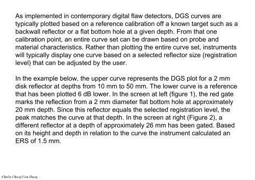
As implemented in contemporary digi
- Page 1595 and 1596:
More reading on DGS
- Page 1597 and 1598:
DGS # of near field
- Page 1599 and 1600:
DGS-If you have a signal feom a fla
- Page 1601 and 1602:
Locating reflectors with an angle-b
- Page 1603 and 1604:
Scanning Patterns
- Page 1605 and 1606:
Scanning Patterns
- Page 1607 and 1608:
Scanning Patterns
- Page 1609 and 1610:
Scanning Patterns
- Page 1611 and 1612:
Scanning Patterns
- Page 1613 and 1614:
Scanning Patterns
- Page 1615 and 1616:
Scanning Patterns
- Page 1617:
Scanning Patterns
- Page 1623 and 1624:
Practice Makes Perfect 81. The 100
- Page 1625 and 1626:
Addendum-01b Equipment Calibration
- Page 1627 and 1628:
The Circuitry: • Voltage activati
- Page 1629 and 1630:
Pulse-Echo Instrumentation Pulser C
- Page 1631 and 1632:
Pulse-Echo Instrumentation The Puls
- Page 1633 and 1634:
Pulse-Echo Instrumentation PULSER T
- Page 1635 and 1636:
Pulse-Echo Instrumentation CLOCK GE
- Page 1637 and 1638:
Pulse-Echo Instrumentation Increasi
- Page 1639 and 1640:
Pulse-Echo Instrumentation The Tran
- Page 1641 and 1642:
PULSER TGC UNIT MEMORY TRX TRS RF R
- Page 1643 and 1644:
Pulse-Echo Instrumentation Electric
- Page 1645 and 1646:
Pulse-Echo Instrumentation Amplitud
- Page 1647 and 1648:
Pulse-Echo Instrumentation Primary
- Page 1649 and 1650:
Pulse-Echo Instrumentation TGC Cont
- Page 1651 and 1652:
Pulse-Echo Instrumentation KNEE MAX
- Page 1653 and 1654:
Pulse-Echo Instrumentation The slid
- Page 1655 and 1656:
Pulse-Echo Instrumentation Frequenc
- Page 1657 and 1658:
Pulse-Echo Instrumentation Wide-ban
- Page 1659 and 1660:
Pulse-Echo Instrumentation DYNAMIC
- Page 1661 and 1662:
Pulse-Echo Instrumentation RF ampli
- Page 1663 and 1664:
Pulse-Echo Instrumentation LOGARITH
- Page 1665 and 1666:
Pulse-Echo Instrumentation R-F ampl
- Page 1667 and 1668:
Pulse-Echo Instrumentation REJECTIO
- Page 1669 and 1670:
Pulse-Echo Instrumentation SIGNAL P
- Page 1671 and 1672:
Pulse-Echo Instrumentation RECTIFIC
- Page 1673 and 1674:
Pulse-Echo Instrumentation Full-Wav
- Page 1675 and 1676:
Pulse-Echo Instrumentation Smoothin
- Page 1677 and 1678:
Pulse-Echo Instrumentation DIGITAL
- Page 1679 and 1680:
Pulse-Echo Instrumentation 4. Digit
- Page 1681 and 1682:
Matrix Columns, y coordinates
- Page 1683 and 1684:
10x 10y X, Y ADDRESS 8x 7y 5x 5y 3x
- Page 1687 and 1688:
X X X X X X X X X X X X
- Page 1689 and 1690:
50 50 50 50 50 50 50 50 50 50 50 50
- Page 1691 and 1692:
Pulse-Echo Instrumentation DIGITAL
- Page 1693 and 1694:
Pulse-Echo Instrumentation Echoes d
- Page 1695 and 1696:
Pulse-Echo Instrumentation Gray Sca
- Page 1697 and 1698:
Pulse-Echo Instrumentation % Availa
- Page 1699 and 1700:
Pulse-Echo Instrumentation 9 7 8 8
- Page 1701 and 1702:
Pulse-Echo Instrumentation Zoom Mag
- Page 1703 and 1704:
Pulse-Echo Instrumentation Data Pre
- Page 1705 and 1706:
65. In Figure 3, transducer A is be
- Page 1707 and 1708:
68. When the incident angle is chos
- Page 1709 and 1710:
Q: In a UT test system where signal
- Page 1711 and 1712:
Q: The intended purpose of the adju
- Page 1716 and 1717:
Trigonometry http://www.mathwarehou
- Page 1718:
1.0 Material Acoustic Properties Ma
- Page 1721 and 1722:
Ultrasonic Formula
- Page 1723 and 1724:
3.0 Properties of Acoustic Plane Wa
- Page 1725 and 1726:
What properties of material affect
- Page 1727 and 1728: Where V is the speed of sound, C is
- Page 1729 and 1730: 5.0 Attenuation The amplitude chang
- Page 1731 and 1732: Attenuation can be determined by ev
- Page 1733 and 1734: Attenuation is generally proportion
- Page 1735 and 1736: 7.0 Acoustic Impedance Sound travel
- Page 1737 and 1738: Reflection/Transmission Energy as a
- Page 1739 and 1740: Using the above applet, note that t
- Page 1741 and 1742: Practice Makes Perfect Following ar
- Page 1743 and 1744: Q2: What is the percentage of sound
- Page 1745 and 1746: Snell’s Law http://education-port
- Page 1747 and 1748: Practice Made Perfect 7. Snell's la
- Page 1749 and 1750: Practice Makes Perfect 11. Calculat
- Page 1751 and 1752: The following formula relates some
- Page 1753 and 1754: 10. Near/ Far Fields http://miac.un
- Page 1757 and 1758: Modified Near Zone T Perspex Modifi
- Page 1759 and 1760: Apparent Near Zone distance
- Page 1761 and 1762: The focal length F is determined by
- Page 1763 and 1764: Calculate the offset for following
- Page 1765 and 1766: 14.0 Inverse Law and Inverse Square
- Page 1768 and 1769: Inverse Law: For large reflector, r
- Page 1770 and 1771: - Distance Gain Size is a method of
- Page 1772 and 1773: In the general diagram the size of
- Page 1774 and 1775: Example: If you has a signal at a c
- Page 1776 and 1777: More on DGS/AVG by Olympus http://w
- Page 1780 and 1781: Figure1:
- Page 1782 and 1783: 15.0 Pulse Repetitive Frequency/Rat
- Page 1784 and 1785: Q4-12 Answer: First calculate the p
- Page 1790 and 1791: Addendum-03 Questions & Answers I C
- Page 1792 and 1793: Make mistakes now, not during exam!
- Page 1794 and 1795: 30. On an A-scan display the dead z
- Page 1796 and 1797: 31. As the acoustic impedance ratio
- Page 1798 and 1799: 15. Which type of test block is use
- Page 1800 and 1801: Mistake Made ----------------------
- Page 1802 and 1803: Question: Which type of screen pres
- Page 1805 and 1806: Table 1.2
- Page 1807 and 1808: Q1-13 The second critical angle at
- Page 1809 and 1810: For evaluating material properties
- Page 1811 and 1812: Q1-22 The beam spread half angle I
- Page 1813 and 1814: Q2-12 An angle beam produce a 45°
- Page 1815 and 1816: Q2-17 A change in echo amplitude fr
- Page 1817 and 1818: Q2-19 What is the rate of attenuati
- Page 1819 and 1820: Q2-11 A change in 16dB on the atten
- Page 1821 and 1822: Q3-7 The half angle beam spread of
- Page 1823 and 1824: Monkey made mistake too!
- Page 1825 and 1826: Smart Himba Girl do not made mistak
- Page 1827 and 1828: Smart Himba Girl do not made mistak
- Page 1829 and 1830:
Q3-8 Answer: The next SDH used will
- Page 1831 and 1832:
Q3-13 During examination, an indica
- Page 1833 and 1834:
Q3-15 In contact testing, the back
- Page 1835 and 1836:
Q4-13 Answer: PRR = number of pulse
- Page 1837 and 1838:
Q4-16
- Page 1839 and 1840:
Q4-17 Illustrations Complete loop=4
- Page 1841 and 1842:
8. When testing a 30 mm diameter, 5
- Page 1843 and 1844:
Q5-20 Answer: None of above
- Page 1845:
Q5-22 Table B-1
- Page 1848 and 1849:
38. The angle of a refracted shear
- Page 1850 and 1851:
48. A more highly damped transducer
- Page 1852 and 1853:
47. When a vertical indication has
- Page 1854 and 1855:
63. The purpose of the couplant is
- Page 1856:
Immersion Testing Method
- Page 1861 and 1862:
Standards Answer: B
- Page 1863 and 1864:
Standards Answer: A (or C?)
- Page 1865 and 1866:
Standards Answer: C
- Page 1867 and 1868:
Standards Answer: C
- Page 1869:
Standards Answer: A?
- Page 1872 and 1873:
Arrows shown standard correct answe
- Page 1874 and 1875:
Arrows shown standard correct answe
- Page 1876:
Arrows shown standard correct answe
- Page 1879 and 1880:
Arrows shown standard correct answe
- Page 1881 and 1882:
Arrows shown standard correct answe
- Page 1883 and 1884:
Take a break mms://a588.l3944020587
- Page 1885 and 1886:
Arrows shown standard correct answe
- Page 1887 and 1888:
Practices Make Perfect
- Page 1889 and 1890:
Click to Q&A http://www.ndtcalc.com
- Page 1891 and 1892:
Ultrasonic Formula
- Page 1893:
Inverse Square Law http://www.cyber
- Page 1896 and 1897:
Echo Amplitude- Reflector Size “D
- Page 1898 and 1899:
Scanning Speed: Scanner speed = (PR
- Page 1900 and 1901:
Expert at Works
- Page 1902 and 1903:
Content: Exercise 1 Exercise 2 Expe
- Page 1904 and 1905:
Practices Make Perfect
- Page 1906 and 1907:
Click to Q&A http://www.ndtcalc.com
- Page 1908 and 1909:
2.0: Ultrasound Formula http://www.
- Page 1910 and 1911:
Ultrasonic Formula
- Page 1912:
Inverse Square Law http://www.cyber
- Page 1915 and 1916:
Echo Amplitude- Reflector Size “D
- Page 1917 and 1918:
Scanning Speed: Scanner speed = (PR
- Page 1919 and 1920:
Offshore Lifts
- Page 1921 and 1922:
Top Scorer
- Page 1923 and 1924:
Exercises Studyblue-01
- Page 1925 and 1926:
3. The only significant sound wave
- Page 1927 and 1928:
7. The simple experiment where a st
- Page 1929 and 1930:
11. The differences in signals rece
- Page 1931 and 1932:
15. Which of the following may resu
- Page 1933 and 1934:
19. When examining materials for pl
- Page 1935 and 1936:
21. Rayleigh waves are influenced m
- Page 1937 and 1938:
25. Which of the following scanning
- Page 1939 and 1940:
29. At an interface between two dif
- Page 1941 and 1942:
33. In the immersion technique, the
- Page 1943 and 1944:
37. On an A-scan display, what repr
- Page 1945 and 1946:
41. A 152 mm (6 in) diameter rod is
- Page 1947 and 1948:
Immersion Testing Bridge Manipulato
- Page 1949 and 1950:
45. Which best describes a typical
- Page 1951 and 1952:
49. During a straight beam ultrason
- Page 1953 and 1954:
53. A smooth flat discontinuity who
- Page 1955 and 1956:
57. The angle at which 90 degrees r
- Page 1957 and 1958:
61. Large gains in a metallic test
- Page 1959 and 1960:
65. In Figure 3, transducer A is be
- Page 1961 and 1962:
69. In Figure 4, transducer B is be
- Page 1963 and 1964:
72. If you were requested to design
- Page 1965 and 1966:
76. The electronic circuitry that a
- Page 1967 and 1968:
80. The angle formed by an ultrason
- Page 1969 and 1970:
83. A grouping of a number of cryst
- Page 1971 and 1972:
85. The angular position of the ref
- Page 1973 and 1974:
89. The change in direction of an u
- Page 1975 and 1976:
93. In general, shear waves are mor
- Page 1977 and 1978:
97. The speed with which ultrasonic
- Page 1979 and 1980:
Barbecue Lamb
- Page 1981 and 1982:
103. If ultrasonic wave is transmit
- Page 1983 and 1984:
107. When inspecting a rolled or fo
- Page 1985 and 1986:
111. During immersion testing of an
- Page 1987 and 1988:
115. One of the most common applica
- Page 1989 and 1990:
119. At a water-steel interface the
- Page 1991 and 1992:
123. In a basic pulse echo ultrason
- Page 1993 and 1994:
127. The instrument displays a plan
- Page 1995 and 1996:
131. The motion of particles in a s
- Page 1997 and 1998:
135. As frequency increases in ultr
- Page 1999 and 2000:
139. The velocity of longitudinal w
- Page 2001 and 2002:
143. A diagram in which the entire
- Page 2003 and 2004:
147. The expansion and contraction
- Page 2005 and 2006:
151. A quartz crystal cut so that i
- Page 2007 and 2008:
153. When an ultrasonic beam reache
- Page 2009 and 2010:
157. The most common used method of
- Page 2011 and 2012:
161. Acoustic velocities of materia
- Page 2013 and 2014:
165. The resolving power of a trans
- Page 2015 and 2016:
169. Because the velocity of sound
- Page 2017 and 2018:
173. In an A-scan presentation, the
- Page 2019 and 2020:
Fiesta
- Page 2021 and 2022:
Choices
- Page 2023 and 2024:
179. Low frequency sound waves are
- Page 2025 and 2026:
Frequency = 5 MHZ, Wavelength λ =
- Page 2027 and 2028:
181. In immersion testing, the acce
- Page 2029 and 2030:
183. In immersion testing, irreleva
- Page 2031 and 2032:
187. The property of certain materi
- Page 2033 and 2034:
191. The lack of parallelism betwee
- Page 2035 and 2036:
195. Reducing the extent of the dea
- Page 2037 and 2038:
199. Attenuation is the loss of the
- Page 2039 and 2040:
203. The most commonly used method
- Page 2041 and 2042:
Chicken & Squid Satay Treats
- Page 2043 and 2044:
1. The wave mode that has multiple
- Page 2045:
Addendum-04C Questions & Answers- I
- Page 2048 and 2049:
Production Island
- Page 2050 and 2051:
At works
- Page 2053 and 2054:
Assorted Exercises
- Page 2055 and 2056:
Q23. Propagation of ultrasonic wave
- Page 2057 and 2058:
Q30. The sum of reflection & transm
- Page 2059 and 2060:
Practice 2: Source: Lavender Intern
- Page 2061 and 2062:
Q3. On a scan display the dead zone
- Page 2063 and 2064:
Q7. In which zone does the amplitud
- Page 2065 and 2066:
Q11. Of an A-scan display what repr
- Page 2067 and 2068:
Q15. The ratio of the velocity of s
- Page 2069 and 2070:
19. The total energy losses occurri
- Page 2071 and 2072:
Other Sources
- Page 2073:
Q47: A major (!) limitation of usin