ComputerAided_Design_Engineering_amp_Manufactur.pdf

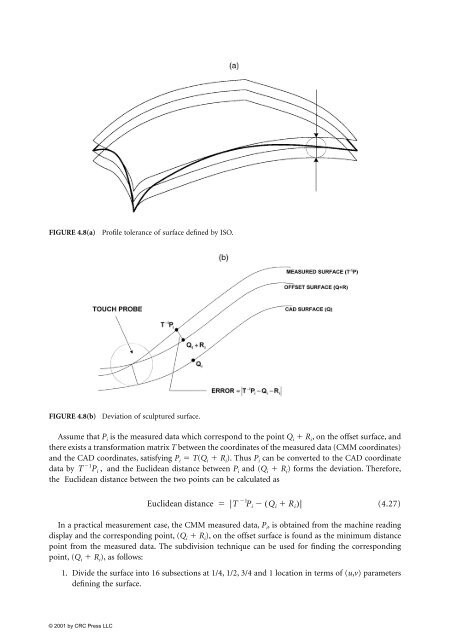
FIGURE 4.8(a) Profile tolerance of surface defined by ISO.
FIGURE 4.8(b) Deviation of sculptured surface.
Assume that Pi is the measured data which correspond to the point Qi � Ri, on the offset surface, and
there exists a transformation matrix T between the coordinates of the measured data (CMM coordinates)
and the CAD coordinates, satisfying Pi � T(Qi � Ri). Thus Pi can be converted to the CAD coordinate
data by T and the Euclidean distance between Pi and (Qi � Ri) forms the deviation. Therefore,
the Euclidean distance between the two points can be calculated as
1 � Pi ,
Euclidean distance |T 1
�
� Pi � Qi � Ri ( )|
(4.27)
In a practical measurement case, the CMM measured data, P i, is obtained from the machine reading
display and the corresponding point, (Q i � R i), on the offset surface is found as the minimum distance
point from the measured data. The subdivision technique can be used for finding the corresponding
point, (Q i � R i), as follows:
1. Divide the surface into 16 subsections at 1/4, 1/2, 3/4 and 1 location in terms of (u,v) parameters
defining the surface.