ComputerAided_Design_Engineering_amp_Manufactur.pdf

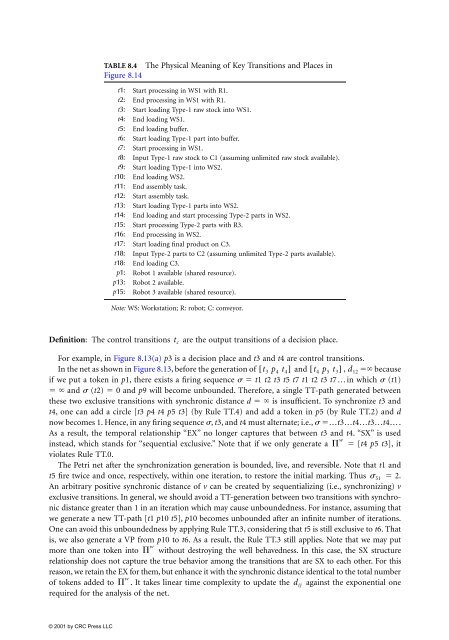
TABLE 8.4 The Physical Meaning of Key Transitions and Places in
Figure 8.14
t1: Start processing in WS1 with R1.
t2: End processing in WS1 with R1.
t3: Start loading Type-1 raw stock into WS1.
t4: End loading WS1.
t5: End loading buffer.
t6: Start loading Type-1 part into buffer.
t7: Start processing in WS1.
t8: Input Type-1 raw stock to C1 (assuming unlimited raw stock available).
t9: Start loading Type-1 into WS2.
t10: End loading WS2.
t11: End assembly task.
t12: Start assembly task.
t13: Start loading Type-1 parts into WS2.
t14: End loading and start processing Type-2 parts in WS2.
t15: Start processing Type-2 parts with R3.
t16: End processing in WS2.
t17: Start loading final product on C3.
t18: Input Type-2 parts to C2 (assuming unlimited Type-2 parts available).
t18: End loading C3.
p1: Robot 1 available (shared resource).
p13: Robot 2 available.
p15: Robot 3 available (shared resource).
Note: WS: Workstation; R: robot; C: conveyor.
t c
Definition: The control transitions are the output transitions of a decision place.
For example, in Figure 8.13(a) p3 is a decision place and t3 and t4 are control transitions.
In the net as shown in Figure 8.13, before the generation of [ t3 p4 t4] and [ t4 p5 t3] , d12 �� because
if we put a token in p1, there exists a firing sequence � � t1 t2 t3 t5 t7 t1 t2 t3 t7…in which � (t1)
� � and � (t2) � 0 and p9 will become unbounded. Therefore, a single TT-path generated between
these two exclusive transitions with synchronic distance d � � is insufficient. To synchronize t3 and
t4, one can add a circle [t3 p4 t4 p5 t3] (by Rule TT.4) and add a token in p5 (by Rule TT.2) and d
now becomes 1. Hence, in any firing sequence �, t3, and t4 must alternate; i.e., � �…t3…t4…t3…t4….
As a result, the temporal relationship “EX” no longer captures that between t3 and t4. “SX” is used
instead, which stands for “sequential exclusive.” Note that if we only generate a � � [t4 p5 t3], it
violates Rule TT.0.
The Petri net after the synchronization generation is bounded, live, and reversible. Note that t1 and
t5 fire twice and once, respectively, within one iteration, to restore the initial marking. Thus � 2.
An arbitrary positive synchronic distance of v can be created by sequentializing (i.e., synchronizing) v
exclusive transitions. In general, we should avoid a TT-generation between two transitions with synchronic
distance greater than 1 in an iteration which may cause unboundedness. For instance, assuming that
we generate a new TT-path [t1 p10 t5], p10 becomes unbounded after an infinite number of iterations.
One can avoid this unboundedness by applying Rule TT.3, considering that t5 is still exclusive to t6. That
is, we also generate a VP from p10 to t6. As a result, the Rule TT.3 still applies. Note that we may put
more than one token into without destroying the well behavedness. In this case, the SX structure
relationship does not capture the true behavior among the transitions that are SX to each other. For this
reason, we retain the EX for them, but enhance it with the synchronic distance identical to the total number
of tokens added to . It takes linear time complexity to update the against the exponential one
required for the analysis of the net.
w
�51 � w
� w
dij