ComputerAided_Design_Engineering_amp_Manufactur.pdf

A ik
� ‘U’ and is in a cycle that has a place with more than one input transition. We now apply the
tool to the synthesis of an automated manufacturing system (Figure 8.11).
Description of a Manufacturing System
This automated manufacturing system consists of the following major components (Table 8.3): two
entries, two exits, five machines, two robots, two automatic guided vehicles (AGV), and related conveyors.
It can produce two types of products. An unlimited source of raw materials is assumed. Once machines,
robots, or AGVs start any operation, they cannot be interrupted until the work is complete. We now
build up a well-behaved PN model.
Modeling and Synthesis Process
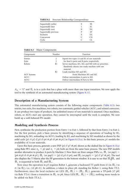
TABLE 8.2 Structure Relationship Correspondence
Sequentially earlier E SE
Sequentially later L SL
Sequentially next N SN
Sequentially previous P SP
Exclusive X EX
Concurrent U CN
Cyclic C CL
TABLE 8.3 Major Components
Components Number Function
Entries 2 Inputs two types (A and B) of raw materials
Exits 2 for final A parts and B parts, respectively.
Robots R1 Serves machines, M1, M2, and M4 with no priorities.
Randomly choose one ready machine with raw
material.
R2 Loads machine M3 and M5.
AGV Systems From Machines M1 and M2
AGV1 Deliver intermediate A parts to M3.
AGV2 Deliver intermediate B Parts to M5.
� i
First, synthesize the production portion from Entry 1 to Exit 1, followed by that from Entry 2 to Exit 2.
For the first portion, pick a basic process by identifying a sequence of operations of loading by R1,
machining by M1, unloading via AGV1, loading by R2, and machining by M3 modeled as shown by the
solid cycle [p1 t1 p2 t2 p3 t3 p4 t4 p5 t5 p6 t6 p1] in Figure 8.12(a). In this basic process, p1 models the
availability of A-raw materials.
Upon this basic process, generate a new PSP [p2 t7 p7 t8 p4] shown as the dashed line in Figure 8.12(a)
using Rule PP.1 since ng � p2 and nj � p4; both are from the same basic process. The new PSP models
another alternative to produce A-parts by Machine 2. Now there are three unique PSPs, i.e., �1 (or psp1) �
[p4 t4 p5 t5 t5 p6 t6 p1], �2 (or psp2) � [p2 t2 p3 t3 p4], and �3 (or psp3) � [p2 t7 p7 t8 p4]. The tool
also displays the T-Matrix after the PP generation in the bottom window. It is easy to see that �2 �3 and
�1 is sequential to both �2 and �3 .
Now since the operation in p3 requires Robot 1, generate a backward TT-path from t2 (in �2 ) to
t1 (in �1), i.e., [t2 p8 t1]. In addition, a token in place p8, standing for Robot 1, using Rule TT.2.
Furthermore, since the local exclusive set LEX (�2, �1 ) � { �2 , �3 }, generate a TP-path [t7 p8]
via Rule TT.4.1 from a transition in �3 to p8. Since LEX( �1 , �2 ) � { �1}, nothing more needs to
be added via Rule TT.4.2.