Fourth Study Conference on BALTEX Scala Cinema Gudhjem
Fourth Study Conference on BALTEX Scala Cinema Gudhjem
Fourth Study Conference on BALTEX Scala Cinema Gudhjem

You also want an ePaper? Increase the reach of your titles
YUMPU automatically turns print PDFs into web optimized ePapers that Google loves.
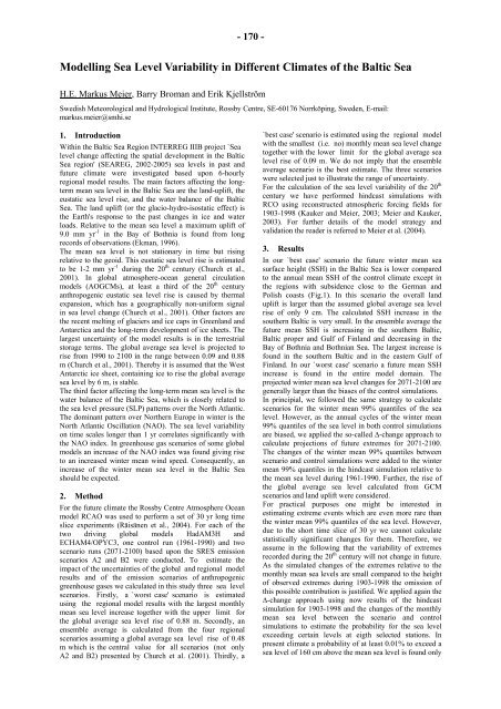
- 170 -<br />
Modelling Sea Level Variability in Different Climates of the Baltic Sea<br />
H.E. Markus Meier, Barry Broman and Erik Kjellström<br />
Swedish Meteorological and Hydrological Institute, Rossby Centre, SE-60176 Norrköping, Sweden, E-mail:<br />
markus.meier@smhi.se<br />
1. Introducti<strong>on</strong><br />
Within the Baltic Sea Regi<strong>on</strong> INTERREG IIIB project `Sea<br />
level change affecting the spatial development in the Baltic<br />
Sea regi<strong>on</strong>' (SEAREG, 2002-2005) sea levels in past and<br />
future climate were investigated based up<strong>on</strong> 6-hourly<br />
regi<strong>on</strong>al model results. The main factors affecting the l<strong>on</strong>gterm<br />
mean sea level in the Baltic Sea are the land-uplift, the<br />
eustatic sea level rise, and the water balance of the Baltic<br />
Sea. The land uplift (or the glacio-hydro-isostatic effect) is<br />
the Earth's resp<strong>on</strong>se to the past changes in ice and water<br />
loads. Relative to the mean sea level a maximum uplift of<br />
9.0 mm yr -1 in the Bay of Bothnia is found from l<strong>on</strong>g<br />
records of observati<strong>on</strong>s (Ekman, 1996).<br />
The mean sea level is not stati<strong>on</strong>ary in time but rising<br />
relative to the geoid. This eustatic sea level rise is estimated<br />
to be 1-2 mm yr -1 during the 20 th century (Church et al.,<br />
2001). In global atmosphere-ocean general circulati<strong>on</strong><br />
models (AOGCMs), at least a third of the 20 th century<br />
anthropogenic eustatic sea level rise is caused by thermal<br />
expansi<strong>on</strong>, which has a geographically n<strong>on</strong>-uniform signal<br />
in sea level change (Church et al., 2001). Other factors are<br />
the recent melting of glaciers and ice caps in Greenland and<br />
Antarctica and the l<strong>on</strong>g-term development of ice sheets. The<br />
largest uncertainty of the model results is in the terrestrial<br />
storage terms. The global average sea level is projected to<br />
rise from 1990 to 2100 in the range between 0.09 and 0.88<br />
m (Church et al., 2001). Thereby it is assumed that the West<br />
Antarctic ice sheet, c<strong>on</strong>taining ice to rise the global average<br />
sea level by 6 m, is stable.<br />
The third factor affecting the l<strong>on</strong>g-term mean sea level is the<br />
water balance of the Baltic Sea, which is closely related to<br />
the sea level pressure (SLP) patterns over the North Atlantic.<br />
The dominant pattern over Northern Europe in winter is the<br />
North Atlantic Oscillati<strong>on</strong> (NAO). The sea level variability<br />
<strong>on</strong> time scales l<strong>on</strong>ger than 1 yr correlates significantly with<br />
the NAO index. In greenhouse gas scenarios of some global<br />
models an increase of the NAO index was found giving rise<br />
to an increased winter mean wind speed. C<strong>on</strong>sequently, an<br />
increase of the winter mean sea level in the Baltic Sea<br />
should be expected.<br />
2. Method<br />
For the future climate the Rossby Centre Atmosphere Ocean<br />
model RCAO was used to perform a set of 30 yr l<strong>on</strong>g time<br />
slice experiments (Räisänen et al., 2004). For each of the<br />
two driving global models HadAM3H and<br />
ECHAM4/OPYC3, <strong>on</strong>e c<strong>on</strong>trol run (1961-1990) and two<br />
scenario runs (2071-2100) based up<strong>on</strong> the SRES emissi<strong>on</strong><br />
scenarios A2 and B2 were c<strong>on</strong>ducted. To estimate the<br />
impact of the uncertainties of the global and regi<strong>on</strong>al model<br />
results and of the emissi<strong>on</strong> scenarios of anthropogenic<br />
greenhouse gases we calculated in this study three sea level<br />
scenarios. Firstly, a `worst case' scenario is estimated<br />
using the regi<strong>on</strong>al model results with the largest m<strong>on</strong>thly<br />
mean sea level increase together with the upper limit for<br />
the global average sea level rise of 0.88 m. Sec<strong>on</strong>dly, an<br />
ensemble average is calculated from the four regi<strong>on</strong>al<br />
scenarios assuming a global average sea level rise of 0.48<br />
m which is the central value for all scenarios (not <strong>on</strong>ly<br />
A2 and B2) presented by Church et al. (2001). Thirdly, a<br />
`best case' scenario is estimated using the regi<strong>on</strong>al model<br />
with the smallest (i.e. no) m<strong>on</strong>thly mean sea level change<br />
together with the lower limit for the global average sea<br />
level rise of 0.09 m. We do not imply that the ensemble<br />
average scenario is the best estimate. The three scenarios<br />
were selected just to illustrate the range of uncertainty.<br />
For the calculati<strong>on</strong> of the sea level variability of the 20 th<br />
century we have performed hindcast simulati<strong>on</strong>s with<br />
RCO using rec<strong>on</strong>structed atmospheric forcing fields for<br />
1903-1998 (Kauker and Meier, 2003; Meier and Kauker,<br />
2003). For further details of the model strategy and<br />
validati<strong>on</strong> the reader is referred to Meier et al. (2004).<br />
3. Results<br />
In our `best case' scenario the future winter mean sea<br />
surface height (SSH) in the Baltic Sea is lower compared<br />
to the annual mean SSH of the c<strong>on</strong>trol climate except in<br />
the regi<strong>on</strong>s with subsidence close to the German and<br />
Polish coasts (Fig.1). In this scenario the overall land<br />
uplift is larger than the assumed global average sea level<br />
rise of <strong>on</strong>ly 9 cm. The calculated SSH increase in the<br />
southern Baltic is very small. In the ensemble average the<br />
future mean SSH is increasing in the southern Baltic,<br />
Baltic proper and Gulf of Finland and decreasing in the<br />
Bay of Bothnia and Bothnian Sea. The largest increase is<br />
found in the southern Baltic and in the eastern Gulf of<br />
Finland. In our `worst case' scenario a future mean SSH<br />
increase is found in the entire model domain. The<br />
projected winter mean sea level changes for 2071-2100 are<br />
generally larger than the biases of the c<strong>on</strong>trol simulati<strong>on</strong>s.<br />
In principial, we followed the same strategy to calculate<br />
scenarios for the winter mean 99% quantiles of the sea<br />
level. However, as the annual cycles of the winter mean<br />
99% quantiles of the sea level in both c<strong>on</strong>trol simulati<strong>on</strong>s<br />
are biased, we applied the so-called ∆-change approach to<br />
calculate projecti<strong>on</strong>s of future extremes for 2071-2100.<br />
The changes of the winter mean 99% quantiles between<br />
scenario and c<strong>on</strong>trol simulati<strong>on</strong>s were added to the winter<br />
mean 99% quantiles in the hindcast simulati<strong>on</strong> relative to<br />
the mean sea level during 1961-1990. Further, the rise of<br />
the global average sea level calculated from GCM<br />
scenarios and land uplift were c<strong>on</strong>sidered.<br />
For practical purposes <strong>on</strong>e might be interested in<br />
estimating extreme events which are even more rare than<br />
the winter mean 99% quantiles of the sea level. However,<br />
due to the short time slice of 30 yr we cannot calculate<br />
statistically significant changes for them. Therefore, we<br />
assume in the following that the variability of extremes<br />
recorded during the 20 th century will not change in future.<br />
As the simulated changes of the extremes relative to the<br />
m<strong>on</strong>thly mean sea levels are small compared to the height<br />
of observed extremes during 1903-1998 the omissi<strong>on</strong> of<br />
this possible c<strong>on</strong>tributi<strong>on</strong> is justified. We applied again the<br />
∆-change approach using now results of the hindcast<br />
simulati<strong>on</strong> for 1903-1998 and the changes of the m<strong>on</strong>thly<br />
mean sea level between the scenario and c<strong>on</strong>trol<br />
simulati<strong>on</strong>s to estimate the probability for the sea level<br />
exceeding certain levels at eigth selected stati<strong>on</strong>s. In<br />
present climate a probability of at least 0.01% to exceed a<br />
sea level of 160 cm above the mean sea level is found <strong>on</strong>ly