CONFINAMIENTO NANOSC´OPICO EN ESTRUCTURAS ... - It works!

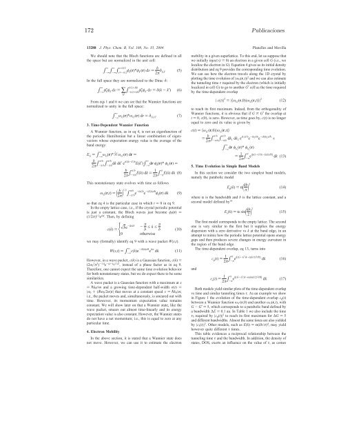
172 Publicaciones13288 J. Phys. Chem. B, Vol. 108, No. 35, 2004 Planelles and MovillaWe should note that the Bloch functions are defined in allthe space but are normalized in the unit cell:∞ ∞∫ -∞∫ -∞∫ x)-b/2In the full space they are normalized to the Dirac δ:From eqs 1 and 6 we can see that the Wannier functions arenormalized to unity in the full space:3. Time-Dependent Wannier FunctionA Wannier function, as in eq 4, is not an eigenfunction ofthe periodic Hamiltonian but a linear combination of eigenvectorswhose expectation energy value is the average of theband energy:This nonstationary state evolves with time as followsso that eq 4 is the particular case in which t ) 0ineq9.In the empty lattice case, i.e., if the crystal periodic potentialis just a constant, the Bloch waves just become φ k(r) )(1/2π) 1/2 e ikr . Then, by definingwe may (formally) identify eq 9 with a wave packet W(x,t).However, in a wave packet, c(k) is a Gaussian function, c(k) )(2σ 0 2 π 3 ) -1/4 e -(k-k 0 )2 /σ 2 , instead of a phase factor as in eq 9.Therefore, one cannot expect the same time evolution behaviorfor both nonstationary states, but we do expect there to be somesimilarities.A wave packet is a Gaussian function with a maximum at x)pk 0t/m and a growing time-dependent half-width σ(t) )|σ 0 + (ipσ 0/2m)t| that moves at a constant speed V)pk 0/m;i.e., the packet moves and, simultaneously, is smeared out withtime. However, its momentum expectation value remainsconstant. We will show later on that a Wannier state, like thewave packet, smears out almost time-linearly and its energyexpectation value is also constant. However, the Wannier statesdo not have a net momentum; i.e., this is equal to zero at anyparticular time.4. Electron Mobilityx)b/2φk (r)*φ k′ (r) dV) b2π δ k,k′ (5)∞∫ / b/2+Hbφk-∞φ k′ dV)∑∫ / φk -b/2+Hbφ k′ dV)δ(k-k′) (6)H∞∫ ωG -∞(r)*ω G′ (r) dr)δ G,G′ (7)∞E G )∫ ωG -∞(r)*Ĥ ω G′ (r) dr)b∫ π/b2π -π/b∫ -π/b dk dk′ e iG(k-k′)b ∞E(k′)∫ -∞ dr φk (r)* φ k′ (r) )b∫ π/b 12π -π/b E(k) dk) ∫ π2π -π E(k) dk (8)ω G (r,t) ) (b2π) 1/2 π/b∫ -π/b e -ikGb e -iE(k)t/p φ k (r) dk (9)c(k)){ be-ikGb- π b e keπ b0 otherwise(10)∞W(x,t) )∫ -∞ c(k)e -iE(k)t/p e ikx dk (11)In the above section, it is stated that a Wannier state doesnot move. However, we can use it to estimate the electronmobility in a given superlattice. To this end, let us suppose thatwe initially inject (t ) 0) an electron in a given cell G (i.e., welocalize the electron in G). Equation 4 gives us its initial densitydistribution and eq 9 provides the corresponding time evolution.We can see how the electron travels along the 1D crystal byplotting the time evolution of |ω G(r,t)| 2 and we can also estimatethe tunneling time τ required by the electron (which is initiallylocalized in cell G) to go to another G′ cell as the time requiredby the time-dependent overlapto reach its first maximum. Indeed, from the orthogonality ofWannier functions, it is obvious that if G * G′ the overlap att ) 0, c(0), is zero. However, as time goes by, c(t) is no longerequal to zero and its value is given by5. Time Evolution in Simple Band ModelsIn this section we consider the two simplest band models,namely the parabolic modelwhere R is the bandwidth and b is the lattice constant, and asecond model defined by 14The first model corresponds to the empty lattice. The secondone is very similar to the first but it supplies the energydispersion with a zero derivative vs k at the band edge, in anattempt to mimic how the periodic lattice potential opens energygaps and then produces severe changes in energy curvature inthe region of the band edge.The time-dependent overlap, eq 13, turns intoand| c(t)| 2 ) |〈ω G′ (r,0)|ω G (r,t)〉| 2 (12)c(t) ) 〈ω G′ (r,0)|ω G (r,t)〉) b ∫ π/b2π -π/b∫ dk1 -π/bdk 2 e ik1G′b e -ik2Gb e -iE(k2)t/p ×∞dr φk1 (r)* φ k2(r)∫ -∞) 1 ∫ π2π -π e i[(G-G′)k-E(k)t/p] dk (13)E p (k) )R (kbπ ) 2 (14)E s (k) )Rsin (kb2 ) 2 (15)c p (t) ) 1 ∫ π2π -π ei[(G-G′)k-R(k/π) 2t/p] dk (16)c s (t)) 1 ∫ π2π -π ei[(G-G′)k-Rsin(k/2) 2t/p] dk (17)Both models yield similar plots of the time-dependent overlapvs time and similar tunneling times τ. As an example we showin Figure 1 the evolution of the time-dependent overlap c p(t)between a Wannier function ω G′(r,0) and another ω G(r,t), withG - G′ ) 5, which corresponds to a parabolic band defined bya bandwidth ∆E ) 0.1 au. In Table 1 we also include the timeτ 5 required by |c p(t)| 2 to reach its first maximum for ∆G ) 5and different bandwidths. Almost the same times are also yieldedby |c s(t)| 2 . Other models, such as E(k) )R(kb/π) 4 , may yieldhowever quite different τ times.This table evidences a reciprocal relationship between thetunneling time τ and the bandwidth. In addition, the density ofstates, DOS, exerts an influence on the value of τ, as comes