CONFINAMIENTO NANOSC´OPICO EN ESTRUCTURAS ... - It works!

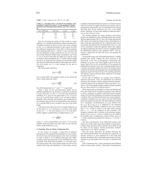
174 Publicaciones13290 J. Phys. Chem. B, Vol. 108, No. 35, 2004 Planelles and MovillaTABLE 2: Tunneling Time τ (To Reach the Neighbor Cell)Calculated Using Eqs 16 and 17 (Corresponding to SimpleParabolic and Sinusoidal Band Models) and Also Using Eq22∆ω)∆E/p (au) π/∆ω (au) τ p (au) τ s (au)0.05 62.8 83 740.1 31.4 41.5 36.71 3.1 4.1 10.710 0.3 0.4 1.1Since by increasing the number of wells results in a largersplitting, 15 we conclude that periodicity reduces tunneling time.It should be pointed out, however, that τ does not just dependon ∆E. As we indicated previously in this section, the DOSalso influences tunneling time. Thus, Table 2 collects tunnelingtimes calculated with eq 22, τ)πp/∆E)π/∆ω, and also fromthe time-dependent overlap coefficient for the two E p(k) andE s(k) energy dispersion models under consideration, eqs 14 and15. As we can see in this table, the simple eq 22 may be usefulto obtain an order of magnitude for τ. To attain a greater insightinto eq 22, we study the time evolution of several band modelswith the same bandwidth and different DOS dispersion models.The E s(k) model, eq 15, is also included for the sake ofcomparison.The linear model, defined byE l (k))R| kb π | (24)has a constant DOS. The quadratic model, eq 14, and the nthpower energy dispersion modelE n (k))R (kbπ ) n (25)have DOS proportional to k -1 and k -(n-1) , respectively.Figure 3 plots, for the abovementioned models and anarbitrary bandwidth of 25 au, the time τ G required by an electronto reach consecutive G cells vs G. We have also included theestimation of τ G given by the approximate eq 22. As can beseen, eq 22 and the linear model, eq 24, are almost indistinguishable.This extremely close behavior can be understood ifwe remember that eq 22 does not include DOS in the estimationof τ G and that DOS is just a constant in the case of the linearmodel.It can also be seen that in the series of models defined by eq25, the slope of τ G vs G decreases as n increases, with a limitof zero as nf∞. The near linearity of τ G vs G in the abovemodels suggests a generalization of (approximate) eq 22:τ G ) a∆E/p G (26)where a ) π for a constant DOS, eq 22, and a ≈ 2 for an idealparabolic band (and almost the same value for the relativelysimilar model defined by eq 15).6. Tunneling Time in Chains of Quantum DotsIn this section we consider a chain built of sphericalhomogeneous InAs quantum dots embedded in a GaAs matrix.Several dot sizes and interdot distances have been consideredin order to obtain a set of different band gaps and widths.Tunneling along the ground and excited minibands have beencalculated. Also chains built of antidots, i.e., two-shell GaAs/InAs nanocrystals with a GaAs barrier-acting core and an InAsexternal well-acting clad embedded in a GaAs matrix, are alsoconsidered. Studying both kinds of systems is of interest becausewhile the electrons are tightly attached to the nanodot center inhomogeneous nanocrystals, they are distributed in the externalshell and, then, loosely attached to the core, in the antidotsystem. Therefore, we may expect different conduction behaviorsin each of the two cases.The isolated quantum dot energy spectrum and electrondensities are obtained by means of the k‚p method and envelopefunction approximation (EFA). 8 Since the energy gap betweenbulk valence and conduction bands in these semiconductors islarge (wide gap semiconductors) the conduction band can besuccessfully described by the one-band model. Then, we carryout the calculations within this approach which only requiresan empirical parameter (the effective mass) to completely definethe Hamiltonian (effective mass approach, EMA 9 ). This parameteris fitted from the bulk and used in the quantum dotcalculations. 16The potential energy part of the k‚p Hamiltonian is a steplikepotential that weakly confines the band electrons in thenanocrystal. In the case of homogeneous nanocrystals, thispotential V(r) is just a well whose height is given by the dotmatrixband off-set (or the electroaffinity of the quantum dotbuilding block material, in the case of isolated quantum dots ina vacuum). In quantum antidots, the well for the electron motionis found in the external clad (and again, the corresponding barrierheights are equal to the band off-sets of the matching materials).The effective masses and band offsets employed in this paperare taken from ref 10.For the sake of simplicity, we consider most symmetric,spherical nanocrystals. Then, the Hamiltonian has sphericalsymmetry and commutes with the angular momentum operator,so that the eigenvectors are labeled as if they were atoms: nL Mz ,where L, M z are the angular quantum numbers (indeed, quantumdots are often referred to as artificial atoms 11 ).When nanocrystals are arranged in a dense one-dimensionalarray, they interact and a lowering of symmetry from sphericalto axial is produced. In parallel, individual discrete nanodotenergy levels develop minibands as the quantum dot superlatticeis formed. Since one-dimensional arrays have axial symmetry,cylindrical coordinates (F,z) are used to solve the Hamiltonianeigenvalue equation numerically. The finite-differences methodon a rectangular two-dimensional (F,z) grid defined from[0,-z max] up to [F max,z max] is employed in the numericalprocedure. Periodic boundary conditions on the z-axis, namelyφ(F,z + b) ) e iqb φ(F,z), where b is the super lattice constantand 0 < q < π/b, are employed for this coordinate. Theboundary conditions that we impose in the directions perpendicularto the z-axis (i.e., on the F coordinate) are the standardfor bounded states of nonperiodic systems, namely, φ(F max,z)) 0 (this condition being replaced by (∂φ/∂F) (0,z) ) 0 for M z )0 states).The above discretization of the differential equation thatdefines our model yields eigenvalue problems of asymmetric,complex, huge, and sparse matrices that have been finally solvedby means of the iterative Arnoldi factorization method 12implemented in the ARPAC package. 13Once the energy dispersions are obtained following theabovementioned procedure, the tunneling time required by anelectron, located in a given quantum dot in the chain (andtherefore described by the corresponding nonstationary Wannierfunction) to go into another dot in the chain is calculated witheq 13.Table 3 summarizes the τ 5 values calculated for three differentchains of nanocrystals, namely: chains built of homogeneous