- Page 1:
CONFINAMIENTO NANOSCÓPICO ENESTRUC
- Page 5 and 6:
AgradecimientosDecía Albert Einste
- Page 7:
A mi madreA la memoria de mi padre
- Page 10 and 11:
viiihigh-correlation electronic reg
- Page 12 and 13:
xric) resolution method proves the
- Page 14 and 15:
xii14. F. Rajadell, J.L. Movilla, M
- Page 16 and 17:
xivcen para moldear a voluntad su e
- Page 18 and 19:
xvideterminar las características
- Page 23 and 24:
Capítulo 1Fundamentos teóricosEl
- Page 25 and 26:
1.1 Modelo k · p 3donde p = −i¯
- Page 27 and 28:
1.1 Modelo k · p 5inversa de la ma
- Page 29 and 30:
1.2 Heteroestructuras. Aproximació
- Page 31 and 32:
1.3 Masa efectiva dependiente de la
- Page 33 and 34:
1.4 Aplicación de un campo magnét
- Page 35 and 36:
1.5 Potenciales monopartícula adic
- Page 37 and 38:
1.6 Integración numérica del hami
- Page 39 and 40:
1.7 Transiciones intrabanda 17Tras
- Page 41 and 42:
1.7 Transiciones intrabanda 19g) [7
- Page 43 and 44:
Capítulo 2Confinamientos espacial
- Page 45 and 46:
23esta aproximación asume implíci
- Page 47 and 48:
2.1 Puntos cuánticos de InAs en ma
- Page 49 and 50:
2.1 Puntos cuánticos de InAs en ma
- Page 51 and 52:
2.1 Puntos cuánticos de InAs en ma
- Page 53 and 54:
2.1 Puntos cuánticos de InAs en ma
- Page 55 and 56:
Capítulo 3Confinamiento periódico
- Page 57 and 58:
3.1 Funciones de Wannier 35otro con
- Page 59 and 60:
3.1 Funciones de Wannier 373.1.1. F
- Page 61 and 62:
3.2 Evolución temporal en modelos
- Page 63 and 64:
3.2 Evolución temporal en modelos
- Page 65 and 66:
3.2 Evolución temporal en modelos
- Page 67 and 68:
3.3 Tiempo de tunneling en cadenas
- Page 69 and 70:
3.3 Tiempo de tunneling en cadenas
- Page 71 and 72:
Capítulo 4Confinamiento magnético
- Page 73 and 74:
51donde m ∗ es la masa efectiva d
- Page 75 and 76:
4.1 Magnetización de puntos y anil
- Page 77 and 78:
4.1 Magnetización de puntos y anil
- Page 79 and 80:
4.1 Magnetización de puntos y anil
- Page 81 and 82:
4.2 Acoplamiento lateral de anillos
- Page 83 and 84:
4.2 Acoplamiento lateral de anillos
- Page 85 and 86:
4.2 Acoplamiento lateral de anillos
- Page 87 and 88:
4.2 Acoplamiento lateral de anillos
- Page 89 and 90:
Capítulo 5Confinamiento dieléctri
- Page 91 and 92:
69Más complicado pero también ana
- Page 93 and 94:
5.1 Validez de la electrodinámica
- Page 95 and 96:
5.2 Interacciones culómbicas en pu
- Page 97 and 98:
5.2 Interacciones culómbicas en pu
- Page 99 and 100:
5.3 Barreras confinantes finitas e
- Page 101 and 102:
5.3 Barreras confinantes finitas e
- Page 103 and 104:
5.3 Barreras confinantes finitas e
- Page 105 and 106:
5.3 Barreras confinantes finitas e
- Page 107 and 108:
5.4 Impurezas dadoras hidrogenoides
- Page 109 and 110:
5.4 Impurezas dadoras hidrogenoides
- Page 111 and 112:
5.4 Impurezas dadoras hidrogenoides
- Page 113 and 114:
5.4 Impurezas dadoras hidrogenoides
- Page 115 and 116:
5.4 Impurezas dadoras hidrogenoides
- Page 117 and 118:
5.4 Impurezas dadoras hidrogenoides
- Page 119 and 120:
5.4 Impurezas dadoras hidrogenoides
- Page 121 and 122:
5.4 Impurezas dadoras hidrogenoides
- Page 123 and 124:
5.4 Impurezas dadoras hidrogenoides
- Page 125 and 126:
5.4 Impurezas dadoras hidrogenoides
- Page 127 and 128:
5.4 Impurezas dadoras hidrogenoides
- Page 129 and 130:
5.5 Estados superficiales inducidos
- Page 131 and 132:
5.5 Estados superficiales inducidos
- Page 133 and 134:
5.5 Estados superficiales inducidos
- Page 135 and 136:
5.5 Estados superficiales inducidos
- Page 137 and 138:
5.5 Estados superficiales inducidos
- Page 139 and 140:
5.5 Estados superficiales inducidos
- Page 141 and 142:
5.5 Estados superficiales inducidos
- Page 143 and 144:
5.5 Estados superficiales inducidos
- Page 145 and 146:
5.5 Estados superficiales inducidos
- Page 147 and 148:
5.5 Estados superficiales inducidos
- Page 149 and 150:
5.5 Estados superficiales inducidos
- Page 151 and 152:
5.5 Estados superficiales inducidos
- Page 153 and 154:
5.5 Estados superficiales inducidos
- Page 155 and 156:
5.5 Estados superficiales inducidos
- Page 157 and 158:
5.5 Estados superficiales inducidos
- Page 159 and 160:
5.5 Estados superficiales inducidos
- Page 161 and 162:
5.5 Estados superficiales inducidos
- Page 163 and 164:
5.5 Estados superficiales inducidos
- Page 165 and 166:
5.5 Estados superficiales inducidos
- Page 167 and 168:
5.5 Estados superficiales inducidos
- Page 169 and 170:
5.5 Estados superficiales inducidos
- Page 171 and 172:
5.5 Estados superficiales inducidos
- Page 173 and 174: 5.5 Estados superficiales inducidos
- Page 175 and 176: Capítulo 6ConclusionesEn esta Tesi
- Page 177 and 178: 155entre los anillos como la orient
- Page 179 and 180: 157fuerte decaimiento de la intensi
- Page 181 and 182: Publicaciones
- Page 183 and 184: Confinamientos espacial y másico
- Page 185 and 186: Confinamientos espacial y másico 1
- Page 187 and 188: Confinamientos espacial y másico 1
- Page 189 and 190: Confinamientos espacial y másico 1
- Page 191 and 192: Confinamiento periódico
- Page 193 and 194: Confinamiento periódico 171J. Phys
- Page 195 and 196: Confinamiento periódico 173Tunneli
- Page 197 and 198: Confinamiento periódico 175Tunneli
- Page 199 and 200: Confinamiento magnético
- Page 201 and 202: Confinamiento magnético 179Symmetr
- Page 203 and 204: Confinamiento magnético 181Aharono
- Page 205 and 206: Confinamiento magnético 183Aharono
- Page 207 and 208: Confinamiento magnético 185Aharono
- Page 209 and 210: Confinamiento magnético 187PHYSICA
- Page 211 and 212: Confinamiento magnético 189MAGNETI
- Page 213 and 214: Confinamiento magnético 191IOP Pub
- Page 215 and 216: Confinamiento magnético 193938Mean
- Page 217 and 218: Confinamiento magnético 195940QRs
- Page 219 and 220: Confinamiento dieléctrico
- Page 221 and 222: Confinamiento dieléctrico 199Compu
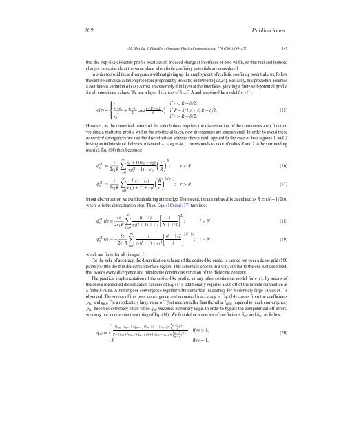
- Page 223: Confinamiento dieléctrico 201146 J
- Page 227 and 228: Confinamiento dieléctrico 205150 J
- Page 229 and 230: Confinamiento dieléctrico 207152 J
- Page 231 and 232: Confinamiento dieléctrico 209PHYSI
- Page 233 and 234: Confinamiento dieléctrico 211OFF-C
- Page 235 and 236: Confinamiento dieléctrico 213OFF-C
- Page 237 and 238: Confinamiento dieléctrico 215OFF-C
- Page 239 and 240: Confinamiento dieléctrico 217PHYSI
- Page 241 and 242: Confinamiento dieléctrico 219BRIEF
- Page 243 and 244: Confinamiento dieléctrico 221PHYSI
- Page 245 and 246: Confinamiento dieléctrico 223TRAPP
- Page 247 and 248: Confinamiento dieléctrico 225Deloc
- Page 249 and 250: Confinamiento dieléctrico 227V s (
- Page 251 and 252: Confinamiento dieléctrico 229with
- Page 253 and 254: Confinamiento dieléctrico 231value
- Page 255 and 256: Confinamiento dieléctrico 233(R in
- Page 257 and 258: Confinamiento dieléctrico 23525R i
- Page 259 and 260: Confinamiento dieléctrico 237monoe
- Page 261 and 262: Confinamiento dieléctrico 239[8] Y
- Page 263 and 264: Confinamiento dieléctrico 241[48]
- Page 265 and 266: Confinamiento dieléctrico 243PHYSI
- Page 267 and 268: Confinamiento dieléctrico 245FROM
- Page 269 and 270: Confinamiento dieléctrico 247PHYSI
- Page 271 and 272: Confinamiento dieléctrico 249THEOR
- Page 273 and 274: Confinamiento dieléctrico 251THEOR
- Page 275 and 276:
Confinamiento dieléctrico 253PHYSI
- Page 277 and 278:
Confinamiento dieléctrico 255DIELE
- Page 279 and 280:
Confinamiento dieléctrico 257DIELE
- Page 281 and 282:
Confinamiento dieléctrico 259DIELE
- Page 283 and 284:
Confinamiento dieléctrico 261DIELE
- Page 285 and 286:
Confinamiento dieléctrico 263PHYSI
- Page 287 and 288:
Confinamiento dieléctrico 265FAR-I
- Page 289 and 290:
Confinamiento dieléctrico 267FAR-I
- Page 291 and 292:
Confinamiento dieléctrico 269Diele
- Page 293 and 294:
Confinamiento dieléctrico 271Diele
- Page 295 and 296:
Confinamiento dieléctrico 273Diele
- Page 297 and 298:
Confinamiento dieléctrico 275Diele
- Page 299 and 300:
Confinamiento dieléctrico 277Diele
- Page 301 and 302:
Confinamiento dieléctrico 279Diele
- Page 303 and 304:
Confinamiento dieléctrico 281Diele
- Page 305 and 306:
Confinamiento dieléctrico 283Diele
- Page 307 and 308:
Confinamiento dieléctrico 285Diele
- Page 309 and 310:
Confinamiento dieléctrico 287Diele
- Page 311 and 312:
Confinamiento dieléctrico 289Diele
- Page 313 and 314:
Confinamiento dieléctrico 291Diele
- Page 315 and 316:
Bibliografía[1] J. Karwowski,“In
- Page 317 and 318:
BIBLIOGRAFÍA 295[23] J.L. Movilla,
- Page 319 and 320:
BIBLIOGRAFÍA 297[48] M.G. Burt,
- Page 321 and 322:
BIBLIOGRAFÍA 299[71] W.H. Press, S
- Page 323 and 324:
BIBLIOGRAFÍA 301[97] U.H. Lee, D.
- Page 325 and 326:
BIBLIOGRAFÍA 303[121] S.W. Chung,
- Page 327 and 328:
BIBLIOGRAFÍA 305[145] R. Blossey y
- Page 329 and 330:
BIBLIOGRAFÍA 307[169] F. Suárez,
- Page 331 and 332:
BIBLIOGRAFÍA 309[194] C. Delerue,
- Page 333 and 334:
BIBLIOGRAFÍA 311[220] J.L. Zhu y X
- Page 335 and 336:
BIBLIOGRAFÍA 313[245] L.M. Peter,
- Page 337 and 338:
BIBLIOGRAFÍA 315[266] P. Rinke, K.
- Page 339 and 340:
BIBLIOGRAFÍA 317[289] Y. Wang, L.
- Page 341 and 342:
BIBLIOGRAFÍA 319[314] A. Wójs y P