Contents - Max-Planck-Institut für Physik komplexer Systeme
Contents - Max-Planck-Institut für Physik komplexer Systeme
Contents - Max-Planck-Institut für Physik komplexer Systeme

Create successful ePaper yourself
Turn your PDF publications into a flip-book with our unique Google optimized e-Paper software.
p(W)<br />
0.1<br />
0.08<br />
0.06<br />
0.04<br />
0.02<br />
0<br />
0.01<br />
0.005<br />
0.001<br />
9900 ∆F<br />
W<br />
10000<br />
Figure 1: Distributions of the work performed during the direct<br />
process (solid lines) and extracted during the time-reversed process<br />
(dashed lines) for various values of the switching rate δλ.<br />
The parameter δλ, the switching rate, controls how<br />
far from equilibrium the system is driven. With fast<br />
switching (red curve on fig. 1), the system is driven further<br />
away from equilibrium than with slow switching<br />
(blue curve). The mean dissipated work is greater, as<br />
are the fluctuations of the work. The maximum work<br />
theorem implies that in the quasi-static limit δλ → 0,<br />
the distributions of the work for the direct and the timereversed<br />
processes both tend towards a Dirac distribution<br />
centered on ∆F .<br />
〈δW(t)〉/δλ<br />
10000<br />
9960<br />
9920<br />
9880<br />
10 −2<br />
5 · 10 −3<br />
10 −3<br />
9840<br />
0 0.2 0.4 0.6 0.8 1<br />
λ(t)<br />
Figure 2: Evolution of the mean work performed (solid lines) and<br />
extracted (dashed lines) 〈 δW<br />
〉 per time step along the direct and re-<br />
δλ<br />
verse processes for different switching rates δλ.<br />
The evolution of the quantity δW<br />
δλ during switching<br />
helps to understand how the distributions in fig. 1<br />
arise. Fig. 2 shows the evolution of its mean value 〈 δW<br />
δλ 〉<br />
along the process for different values of the switching<br />
rate δλ. Examples of the fluctuations of δW<br />
δλ around its<br />
mean value are shown on fig. 3. The mean value of δW<br />
δλ<br />
during the direct and the reverse process are very close<br />
to one another for a slow process and further apart for<br />
a fast one, implying an increase in the mean dissipated<br />
work as the switching rate increases. The amplitude of<br />
the fluctuations of δW<br />
δλ are not influenced by the switching<br />
rate. However, for slow switching (red curve on<br />
fig. 3), the system has more time to fluctuate and the<br />
fluctuations are partly averaged out when performing<br />
the integration (4).<br />
δW(t)−〈δW(t)〉<br />
δλ<br />
80<br />
40<br />
0<br />
-40<br />
-80<br />
10 −4<br />
10 −3<br />
0 0.2 0.4 0.6 0.8 1<br />
λ(t)<br />
Figure 3: Fluctuations of δW<br />
δλ<br />
along the process for two values of δλ.<br />
For Gaussian distributions of the dissipated work Wd<br />
one can easily verify that Crooks’ relation (1) implies<br />
that the mean value W d and variance σ 2 of the dissipated<br />
work for the direct and the time-reversed processes<br />
coincide. Crooks’ relation then reduces to a generalized<br />
fluctuation-dissipation relation [4]:<br />
σ 2 = 2kBT W d<br />
Fig. 4 shows the distribution of the quantity Wd =<br />
Wd/σ − σ/2kBT for the direct and the time-reversed<br />
process for various values of the switching rate. This<br />
quantity has a Gaussian distribution with zero mean<br />
and unit variance for all values of the switching rate,<br />
implying that the dissipated work Wd has a Gaussian<br />
distribution and satisfies (6) and therefore Crooks’ relation<br />
(1) as well.<br />
p( p( Wd ) p( Wd ) p( Wd ) p( Wd ) p( Wd ) p( Wd ) p( Wd ) p( Wd ) p( Wd ) p( Wd ) p( Wd ) p( Wd ) p( Wd ) p( Wd ) Wd )<br />
100 100 100 100 100 100 100 100 100 100 100 100 100 100 100 10−1 10−1 10−1 10−1 10−1 10−1 10−1 10−1 10−1 10−1 10−1 10−1 10−1 10−1 10−1 10−2 10−2 10−2 10−2 10−2 10−2 10−2 10−2 10−2 10−2 10−2 10−2 10−2 10−2 10−2 10−3 10−3 10−3 10−3 10−3 10−3 10−3 10−3 10−3 10−3 10−3 10−3 10−3 10−3 10−3 10−4 10−4 10−4 10−4 10−4 10−4 10−4 10−4 10−4 10−4 10−4 10−4 10−4 10−4 10−4 10−5 10−5 10−5 10−5 10−5 10−5 10−5 10−5 10−5 10−5 10−5 10−5 10−5 10−5 10−5 10−6 10−6 10−6 10−6 10−6 10−6 10−6 10−6 10−6 10−6 10−6 10−6 10−6 10−6 10−6 -6 -4 -2 0 W W W W W W W W W W W W W W W d<br />
2 4 6<br />
Figure 4: Distribution of the quantity f Wd = Wd/σ −σ/2kBT for the<br />
direct and reverse process for various values of δλ.<br />
A more careful analysis of the fluctuations suggests<br />
that these are equilibrium heat bath fluctuations in<br />
which only the mean value depends of the protocol and<br />
hence reflects the distance from equilibrium. It is evident<br />
that this cannot hold for arbitrary situations, in<br />
particular not in cases where the driving force creates<br />
dynamical instabilities. The details are still awaiting<br />
further investigation. This issue is relevant for macroscopic<br />
fluctuations in non-equilibrium systems that are<br />
close to the thermodynamic limit, for which pure heat<br />
bath fluctuations should become invisible.<br />
[1] H. B. Callen, THERMODYNAMICS AND AN INTRODUCTION TO<br />
THERMOSTATISTICS, John Wiley & sons (1985).<br />
[2] G. E. Crooks, J. of Stat. Phys. 90 (1998) 1481.<br />
[3] R. Adhikari et al, Europys. Lett. 71 (2005) 473; B. Dünweg,<br />
U. D. Schiller and A. J. C. Ladd, Phys. Rev. E 76 (2007) 036704.<br />
[4] L. Granger, M. Niemann and H. Kantz, J. Stat. Mech.: Th. and<br />
Exp. (2010) P06029<br />
2.14. Work Dissipation Along a Non Quasi-Static Process 69<br />
(6)