Contents - Max-Planck-Institut für Physik komplexer Systeme

2.26 Shortcuts to Adiabaticity in Quantum Systems
J. GONZALO MUGA, E. TORRONTEGUI, A. RUSCHHAUPT, D. GUÉRY-ODELIN
Introduction. An “adiabatic process” in quantum
mechanics is a slow change of Hamiltonian parameters
that keeps the populations of the instantaneous eigenstates
constant. These processes are frequently used to
drive or prepare states in a robust and controllable way,
and have also been proposed to solve complicated computational
problems, but they are, by definition, slow.
Our objective is to find “shortcuts to adiabaticity”, cutting
down the time to arrive at the same final state. We
have proposed different ways to achieve this goal for
general or specific cases based on Lewis-Riesenfeld invariants
and inverse engineering [1].
A different approach to shortcuts to adiabaticity is due
to Berry [2]. He has proposed a Hamiltonian H(t) for
which the adiabatic approximation of the state evolution
under a time-dependent reference Hamiltonian
H0(t) becomes the exact dynamics with H(t). This
has been applied at least formally to spins in magnetic
fields, harmonic oscillators, or to speed up adiabatic
state-preparation methods such as Rapid Adiabatic
Passage (RAP), Stimulated Rapid Adiabatic Passage
(STIRAP) and its variants [3].
Basic theory. A one-dimensional Hamiltonian with
an invariant which is quadratic in momentum must
have the form H = p 2 /2m + V (q,t), with the potential
(see [4] for details)
V (q,t) = −F(t)q+ m
2 ω2 (t)q 2 + 1
U
ρ(t) 2
q − α(t)
ρ(t)
. (1)
ρ, α, ω, and F are arbitrary functions of time that satisfy
two auxiliary equations
¨ρ + ω 2 (t)ρ = ω2 0
ρ 3 , ¨α + ω2 (t)α = F(t)/m, (2)
with ω0 constant. The quadratic dynamical invariants,
up to a constant factor, are given by
1
I = [ρ(p − m ˙α) − m ˙ρ(q − α)]2
2m
+ 1
2 mω2 2
q − α q − α
0 + U . (3)
ρ ρ
We may expand any wavefunction ψ(t) in terms of constant
coefficients cn and eigenvectors ψn (n = 0,1,2...)
of I multiplied by Lewis-Riesenfeld phase factors e iαn .
The basic strategy of invariant-based inverse engineering
methods is to design ρ and α first to achieve desired
objectives, and deduce the Hamiltonian afterwards. In
most applications so far the key point is to control
the boundary conditions of the auxiliary functions and
their time derivatives at initial and final times. In particular,
they may be set so that the eigenvectors of H
and I coincide at initial and final times, and the process
produces no final excitation. It is however not adiabatic,
as excitations are allowed at intermediate times.
Fast expansions. Performing fast expansions of
trapped atoms without losses or vibrational excitation
is important, for example to reduce velocity dispersion
and collisional shifts in spectroscopy and atomic
clocks, to reach extremely low temperatures unaccessible
by standard cooling techniques or, in experiments
with optical lattices, to broaden the atomic cloud before
turning on the lattice. Trap contractions are also
common to prepare the state. For a harmonic oscillator
trap we may consider these expansion or contraction
processes by setting α = U = F = 0. Once ρ(t) is designed
to make H(t) and I(t) commute at the boundary
times, with frequencies ω0 and ωf , we get ω(t) from (2).
This has been implemented experimentally to decompress
87 Rb cold atoms in a harmonic magnetic trap [5].
The extension to Bose-Einstein condensates may be carried
out with a variational ansatz and has been realized
experimentally too [5]. This poses in principle no fundamental
lower limit to the final time tf , which could
be arbitrarily small, but for short enough tf , ω(t) may
become purely imaginary at some t [1], which corresponds
to a parabolic repeller configuration. Also, the
energy required may be too high, as analyzed next.
Ω fHz
0.5
0.4
0.3
0.2
0.1
125
45
85
5
0.0
0.00 0.01 0.02 0.03 0.04 0.05
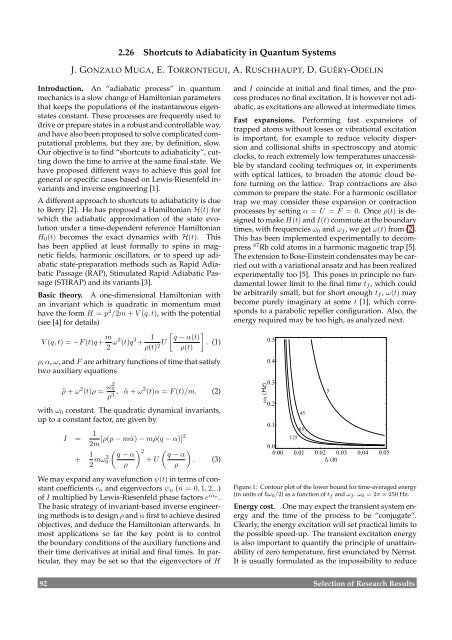
tfs Figure 1: Contour plot of the lower bound for time-averaged energy
(in units of ω0/2) as a function of tf and ωf . ω0 = 2π × 250 Hz.
Energy cost. One may expect the transient system energy
and the time of the process to be “conjugate”.
Clearly, the energy excitation will set practical limits to
the possible speed-up. The transient excitation energy
is also important to quantify the principle of unattainability
of zero temperature, first enunciated by Nernst.
It is usually formulated as the impossibility to reduce
92 Selection of Research Results