Structural Health Monitoring Using Smart Sensors - ideals ...
Structural Health Monitoring Using Smart Sensors - ideals ...
Structural Health Monitoring Using Smart Sensors - ideals ...

Create successful ePaper yourself
Turn your PDF publications into a flip-book with our unique Google optimized e-Paper software.
Power spectral densities (g 2 /Hz)<br />
10 0 Imote2 1<br />
Imote2 2<br />
Reference 1<br />
Reference 2<br />
10 -2<br />
10 -4<br />
10 -6<br />
Power spectral densities (g 2 /Hz)<br />
10 0<br />
10 -2<br />
10 -4<br />
Imote2 1<br />
Imote2 2<br />
10 -6<br />
Reference 1<br />
Reference 2<br />
0 20 40 60 80 100 120 140 0 20 40 60 80 100 120 140<br />
Frequency (Hz)<br />
Frequency (Hz)<br />
(a) longitudinal<br />
(b) transverse<br />
Power spectral densities (g 2 /Hz)<br />
10 0<br />
10 -2<br />
10 -4<br />
Imote2 1<br />
10 -6<br />
Imote2 2<br />
Reference 1<br />
Reference 2<br />
0 20 40 60 80 100 120 140<br />
Frequency (Hz)<br />
(c) vertical<br />
Figure 7.16. Acceleration power spectral densities of Imote2s and reference sensors.<br />
The same observation is made when the signals are compared in terms of power<br />
spectral density (see Figure. 7.16). Note that signals above 100 Hz cannot be directly<br />
comparable because the cutoff frequencies of filters involved are set around 100 Hz. As<br />
with the time domain comparison, the power spectral density of the longitudinal<br />
accelerations shows differences between the two Imote2 signals. The observable<br />
difference in the signals is not constant over frequency. Another finding from the plot for<br />
the longitudinal acceleration is that Imote2s gives smaller signal magnitude above 80 Hz<br />
than PCB accelerometers. In general, the Imote2 signals are close to each other.<br />
Transfer functions between the Imote2 accelerometers, between reference<br />
accelerometers, and between the Imote2 and reference accelerometers are then estimated<br />
(see Figure 7.17). The transfer function magnitude plotted against frequency reveals<br />
differences in the sensitivities of two signals as a function of frequency. As can be seen in<br />
Figure 7.17, the transfer function magnitude for the vertical acceleration is nearly flat<br />
below 100 Hz. The compared sets of signals are considered close to each other confirming<br />
findings from Figures 7.15 and 7.16. The fluctuation found around 30 Hz, as well as<br />
fluctuation in low-frequency range, is considered to be due to the signals being extremely<br />
small, as shown in Figure 7.16. Transfer functions for the transverse acceleration confirm<br />
115