Structural Health Monitoring Using Smart Sensors - ideals ...

Node 1
x1
i =1,2,…,ns
E
x 1 t x i
t
Node 2
Node 3
Node 4
Node 5
x2
x3
x4
x5
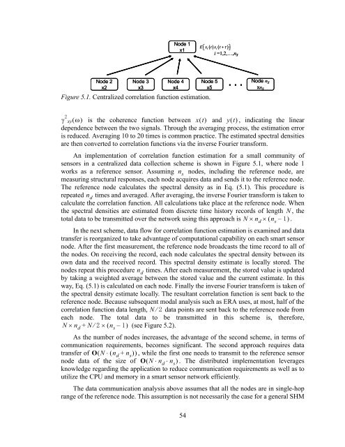
Figure 5.1. Centralized correlation function estimation.
. . .
Node ns
xns
xy is the coherence function between xt and yt , indicating the linear
dependence between the two signals. Through the averaging process, the estimation error
is reduced. Averaging 10 to 20 times is common practice. The estimated spectral densities
are then converted to correlation functions via the inverse Fourier transform.
An implementation of correlation function estimation for a small community of
sensors in a centralized data collection scheme is shown in Figure 5.1, where node 1
works as a reference sensor. Assuming n s
nodes, including the reference node, are
measuring structural responses, each node acquires data and sends it to the reference node.
The reference node calculates the spectral density as in Eq. (5.1). This procedure is
repeated n d
times and averaged. After averaging, the inverse Fourier transform is taken to
calculate the correlation function. All calculations take place at the reference node. When
the spectral densities are estimated from discrete time history records of length N , the
total data to be transmitted over the network using this approach is N
n d
n s
– .
In the next scheme, data flow for correlation function estimation is examined and data
transfer is reorganized to take advantage of computational capability on each smart sensor
node. After the first measurement, the reference node broadcasts the time record to all of
the nodes. On receiving the record, each node calculates the spectral density between its
own data and the received record. This spectral density estimate is locally stored. The
nodes repeat this procedure n d
times. After each measurement, the stored value is updated
by taking a weighted average between the stored value and the current estimate. In this
way, Eq. (5.1) is calculated on each node. Finally the inverse Fourier transform is taken of
the spectral density estimate locally. The resultant correlation function is sent back to the
reference node. Because subsequent modal analysis such as ERA uses, at most, half of the
correlation function data length, N data points are sent back to the reference node from
each node. The total data to be transmitted in this scheme is, therefore,
N
n d
+ N n s
–
(see Figure 5.2).
As the number of nodes increases, the advantage of the second scheme, in terms of
communication requirements, becomes significant. The second approach requires data
transfer of ON
n d
+ n s
, while the first one needs to transmit to the reference sensor
node data of the size of ON
n d n s .
The distributed implementation leverages
knowledge regarding the application to reduce communication requirements as well as to
utilize the CPU and memory in a smart sensor network efficiently.
The data communication analysis above assumes that all the nodes are in single-hop
range of the reference node. This assumption is not necessarily the case for a general SHM
54