Structural Health Monitoring Using Smart Sensors - ideals ...

Timer firing every T3
110 data points from sensing driver
T3 T3 T3 T3
t 1
t 2
t 3
t 4
t 5
t 6
t 7
t 8
t
…
n
110 110 110 110 110 110 110 110 110
Start a
sensing task
Start storing
data
Data copied to an array
Check for
sensing
failure
t1 t1+T1 t1+T2 t1+T4
Time
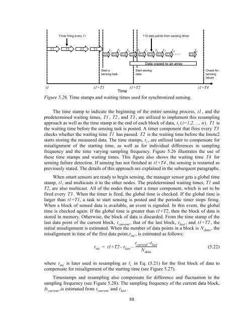
Figure 5.26. Time stamps and waiting times used for synchronized sensing.
The time stamp to indicate the beginning of the entire sensing process, t1 , and the
predetermined waiting times, T1 , T2 , and T3 , are utilized to implement this resampling
approach as well as the time stamp at the end of each block of data, t i
i=1,2, ..., n. T1 is
the waiting time before the sensing task is posted. A timer component that fires every T3
checks whether the waiting time T1 has passed. T2 is the waiting time before the Imote2
starts storing the measured data. The time stamps, t i
, are utilized later to compensate for
misalignment of the starting time, as well as for individual differences in sampling
frequency and the time varying sampling frequency. Figure 5.26 illustrates the use of
these time stamps and waiting times. This figure also shows the waiting time T4 for
sensing failure detection. If sensing has not finished at t1+T4 , the sensing is restarted as
previously stated. The details of this approach are explained in the subsequent paragraphs.
When smart sensors are ready to begin sensing, the manager sensor gets a global time
stamp, t1, and multicasts it to the other nodes. The predetermined waiting times, T1 and
T2, are also multicast. All of the nodes then start a timer component, which is set to be
fired every T3 . When the timer is fired, the global time is checked. If the global time is
larger than t1+T1, a task to start sensing is posted and the periodic timer stops firing.
When a block of sensed data is available, an event is signaled. In this event, the global
time is checked again. If the global time is greater than t1+T2, then the block of data is
stored in memory. Otherwise, the block of data is discarded. From the time stamp of the
last data point of the current block, t current
, that of the last block, t last
, and t1+T2 , the
initial misalignment is estimated. When the number of data points in a block is N data
, the
misalignment in time of the first data point, , is estimated as follows:
t ini
= t1+T2–
t last
t ini
t current
– t last
– --------------------------
N data
88
(5.22)
where t ini
is later used in resampling as l i
in Eq. (5.21) for the first block of data to
compensate for misalignment of the starting time (see Figure 5.27).
Timestamps and resampling also compensate for difference and fluctuation in the
sampling frequency (see Figure 5.28). The sampling frequency of the current data block,
fs current
,is estimated from t current
and t last
.