Structural Health Monitoring Using Smart Sensors - ideals ...

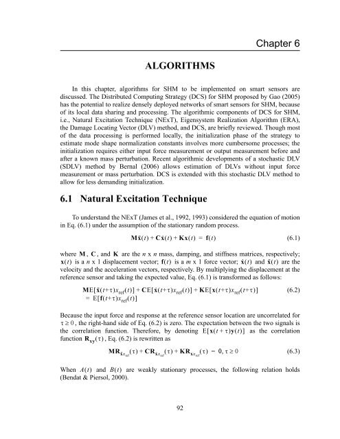
Chapter 6
ALGORITHMS
In this chapter, algorithms for SHM to be implemented on smart sensors are
discussed. The Distributed Computing Strategy (DCS) for SHM proposed by Gao (2005)
has the potential to realize densely deployed networks of smart sensors for SHM, because
of its local data sharing and processing. The algorithmic components of DCS for SHM,
i.e., Natural Excitation Technique (NExT), Eigensystem Realization Algorithm (ERA),
the Damage Locating Vector (DLV) method, and DCS, are briefly reviewed. Though most
of the data processing is performed locally, the initialization phase of the strategy to
estimate mode shape normalization constants involves more cumbersome processes; the
initialization requires either input force measurement or output measurement before and
after a known mass perturbation. Recent algorithmic developments of a stochastic DLV
(SDLV) method by Bernal (2006) allows estimation of DLVs without input force
measurement or mass perturbation. DCS is extended with this stochastic DLV method to
allow for less demanding initialization.
6.1 Natural Excitation Technique
To understand the NExT (James et al., 1992, 1993) considered the equation of motion
in Eq. (6.1) under the assumption of the stationary random process.
Mx·· t
+ Cx· t + Kx
t = f
t
(6.1)
where M , C, and K are the n x n mass, damping, and stiffness matrices, respectively;
x
t is a n x 1 displacement vector; f
t is a m x 1 force vector; x· t and x·· t are the
velocity and the acceleration vectors, respectively. By multiplying the displacement at the
reference sensor and taking the expected value, Eq. (6.1) is transformed as follows:
ME x·· t+x ref t + CEx· t+x ref t + KExt+x ref t+
= Eft+x ref
t
(6.2)
Because the input force and response at the reference sensor location are uncorrelated for
, the right-hand side of Eq. (6.2) is zero. The expectation between the two signals is
the correlation function. Therefore, by denoting Ext
+ y
t as the correlation
function R xy
, Eq. (6.2) is rewritten as
MR x··xref
+ CR x· xref
+ KR xxref
=
(6.3)
When At and Bt are weakly stationary processes, the following relation holds
(Bendat & Piersol, 2000).
92