ClimateChange Assessment Guide.pdf - University of Waterloo

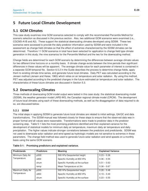
Appendix E E-29Subwatershed 19 Case Study This case study examines nine GCM scenarios selected to comply with the recommended Percentile Method forscenario selection as discussed in the previous section. Also, two additional GCM scenarios were examined (i.e.,CGCM3-A1B and A2). These support the statistical downscaling climates developed using SDSM. These twoscenarios were accessed to provide the daily predictor information used by SDSM and were included in theassessment as change field climates so that the effect of extremes characterized by the SDSM climates can bedetermined. Therefore 11 GCM scenarios in total have been selected for application to change field type climategeneration in this study; the nine scenarios for the Percentile Method and the two for the downscaling method.Change fields are determined for each GCM scenario by determining the differences between average climate valuesfor two different time horizons on a monthly basis. If climate change exists between the time periods then significantdifferences in these values will be apparent. The average climate value for each parameter of interest is contained ina separate GCM temporal file. Section 6.5.2 in the Guide describes the process to determine change fields, applythem to existing climate time series, and generate future local climates. Daily PET was calculated according to theJensen method (Jensen and Haise, 1963) which relies on air temperature and solar radiation. By using this method,PET was adjusted according to the predicted changes in the future estimated air temperature and solar radiation. Thecharacteristics of these future climates are discussed in Section 5.3. Three methods of downscaling GCM model output were tested in this case study: the statistical downscaling model(SDSM), the weather generator model LARS-WG, the Canadian regional climate model (CRCM). The developmentof future local climates using each of these downscaling methods, as well as the disaggregation of data required to doso, are discussed below. The initial steps in applying SDSM to generate future local climates are related to initial settings, QA/QC and datatransformations. The SDSM manual was followed closely for these steps to ensure that the observed data was inproper format and all values were reasonable. Transformations were made to predictor data in the predictorscreening step. Table 5-1 lists the most promising predictors identified and their explained variance for thedevelopment of statistical models for minimum daily air temperature, maximum daily air temperature and dailyprecipitation. The higher values indicate stronger correlations between the predictors and predictands. SDSM wasnot used to downscale solar radiation and wind speed as hydrologic models are not sensitive to extremes in theseparameters. The change field method was used to generate future solar radiation and wind speeds on a monthlybasis using the same GCM scenario.Table 5-1: Promising predictors and explained variance.Predictands Predictors Meaning Explained VarianceMinimum Daily AirTemperaturep500s850shumtempp500s850shum500 hPa Geopotential heightSpecific Humidity at 850 hPaSpecific Humidity at the surfaceMean Temperature at 2m.500 hPa Geopotential heightSpecific Humidity at 850 hPaSpecific Humidity at the surface0.23 – 0.380.36 – 0.550.51 – 0.630.38 – 0.670.28 – 0.480.19 – 0.400.23 – 0.55Maximum Daily AirTemperature