ClimateChange Assessment Guide.pdf - University of Waterloo

More documents

Recommendations

Info

Guide for Assessment of Hydrologic Effects of Climate Change in Ontario22et al., 2008), or whether the assumption that GCMs thatreplicate current climate well will also perform well inprojecting future climate.GCMs have been one of the most commonly usedresources for developing changed climate input datafor water resource impact assessments. Methods usedrange from those that rely entirely on the GCM tomodify historic time series on a monthly average basis(i.e., change field or delta method) through to those thatuse the GCM output to inform local climate modellingtools/approaches (see Chapter 4). In any case, griddedoutput from GCMs is not suitable for direct use inhydrologic models. The GCM resolution, usually on theorder of several hundred kilometres and poor reliabilityat a single time step at a particular grid point, precludeusing these data directly to represent present-day andfuture climates. The change field method is outlined inSections 4.1 and 6.5.2.“Our understanding of climate is still insufficient tojustify proclaiming any one model “best” or evenshowing metrics of model performance that implyskill in predicting the future. More appropriate in anyassessments focusing on [climate change] adaptationor mitigation strategies is to take into account, in apertinently informed manner, the products of distinctmodels built using different expert judgements atcenters around the world” (Bader et al., 2008 11).Essentially, the current recommendation is that climatechange impact assessment should use as manyscenarios of climate change as possible to cover awide range of potential outcomes; scenarios can bederived from differences in climate model formulationsor differences in emission scenarios that drive theclimate response. This point is crucial to developing anunbiased assessment, understanding the uncertaintiessurrounding future climate estimation and developingadaptation strategies that improve resilience to a widerange of future stresses.3.2 GHG Emission Scenarios“Future greenhouse gas (GHG) emissions are theproduct of very complex dynamic systems, determinedby driving forces such as demographic development,socio-economic development, and technologicalchange. Their future evolution is highly uncertain.Scenarios are alternate images of how the future mightunfold and are an appropriate tool to analyse howdriving forces may influence future emission outcomesand to assess associated uncertainties” (Nakicenovicet al., 2000 3).defEmission scenario • plausible representationof the future development of emissions ofsubstances that are potentially radiatively active(e.g., GHGs, aerosols), based on a coherent andinternally consistent set of assumptions aboutdriving forces (such as demographic and socioeconomicdevelopment, technological change)and their key relationships; concentrationscenarios, derived from emission scenarios, areused as input in a climate model [e.g., GCM] tocompute climate projections (Baede et al., 2007)Early modelling of the sensitivity of the climate systemto increasing GHGs was based on equilibrium doublingor quadrupling of carbon dioxide (2xCO 2, 4xCO 2)experiments. As the climate models developed intothe transient response, coupled atmosphere-oceanGCMs, the emission scenarios also evolved. In 1992,the IPCC developed six alternative emission scenariosthat included GHG increase only and GHG (CO 2) andsulphate aerosols combined (the IS92). The IS92a(“business as usual”) scenario represented a mid-rangescenario; emissions were based on historical increasesuntil 1990 then compounded annually at a rate of 1% peryear (Leggett et al., 1992). Although IS92a was the mostfrequently used emission scenario for climate modelsimulations, the IPCC recommended using all six IS92emission scenarios to capture the range of uncertainty infuture emissions (Barrow, 2002).In 2000, the IPCC Special Report on Emission Scenarios(SRES) published a set of new emission scenarios(Nakicenovic et al., 2000). The SRES scenarios werethe “most comprehensive, ambitious, and carefullydocumented emission scenarios produced to date” andpresented a “substantial advance from prior scenarios”(Parson et al., 2007 34). There were 40 SRES scenariosin total, each covering a range of GHG and sulphuremissions identified in the literature and the SRESscenario database (Nakicenovic et al., 2000). These newscenarios contributed to both the IPCC Third and Fourth
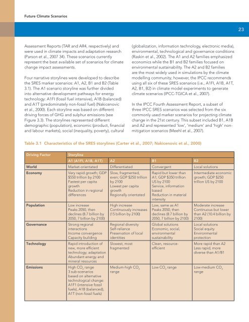
Future Climate Scenarios23Assessment Reports (TAR and AR4, respectively) andwere used in climate impacts and adaptation research(Parson et al., 2007 34). These scenarios currentlyrepresent the best available set of scenarios for climatechange impact assessments.Four narrative storylines were developed to describethe SRES marker scenarios: A1, A2, B1 and B2 (Table3.1). The A1 scenario storyline was further dividedinto alternative development pathways for energytechnology: A1FI (fossil fuel intensive), A1B (balanced)and A1T (predominately non-fossil fuel) (Nakicenovicet al., 2000). Each storyline was based on differentdriving forces of GHG and sulphur emissions (seeFigure 3.3). The storylines represented differentdemographic (population), economic (product, financialand labour markets), social (inequality, poverty), cultural(globalization, information technology, electronic media),environmental, technological and governance conditions(Raskin et al., 2002). The A1 and A2 families emphasizedeconomics while the B1 and B2 families focused onenvironmental sustainability. The A2 and B2 familiesare the most widely used in simulations by the climatemodelling community; however, the IPCC recommendsusing all six of these SRES scenarios (i.e., A1FI, A1B, A1T,A2, B1, B2) in climate model experiments to generateclimate scenarios (IPCC-TGICA et al., 2007).In the IPCC Fourth Assessment Report, a subset ofthree IPCC SRES scenarios was selected from the sixcommonly used marker scenarios for projecting climatechange in the 21st century. This subset included B1, A1Band A2 and represented ‘low’, ‘medium’ and ‘high’ nonmitigationscenarios (Meehl et al., 2007).Table 3.1 Characteristics of the SRES storylines (Carter et al., 2007; Nakicenovic et al., 2000)Driving Factor StorylineA1 (A1FI, A1B, A1T) A2 B1 B2World Market-orientated Differentiated Convergent Local solutionsEconomyVery rapid growth; GDP$550 trillion by 2100Fastest per capitagrowthReduction in regionaldifferencesSlow, fragmented,even; GDP $250 trillionby 2100Lowest per capitagrowthRegionally orientatedRapid but lower thanA1; GDP $350 trillionUS by 2100Service, informationbasedReduction in materialintensityIntermediate economicgrowth; GDP $250trillion US by 2100PopulationGovernanceTechnologyEmissionsLow increasePeaks 2050, thendeclines (8.7 billion by2050, 7 billion by 2100)Strong regionalinteractionsIncome convergenceCapacity buildingRapid introduction ofnew, more efficienttechnology; adaptationAbundant energy andmineral resourcesHigh CO 2range3 sub-scenariosbased on alternativetechnological change:A1F1 (intensive fossilfuels), A1B (balanced),A1T (non-fossil fuels)High increaseContinuously increases(15 billion by 2100)Regional diversitySelf-reliancePreservation of localidentitiesSlowest, mostfragmentedMedium-high CO 2rangeLow, same as A1Peaks 2050, thendeclines (8.7 billion by2050, 7 billion by 2100)Global solutionsEconomic, social,environmentalsustainabilityClean, resourceefficientModerate increaseContinuous but lowerthan A2 (10.4 billion by2100)Local solutionsSocial equityEnvironmentalprotectionMore rapid than A2Less rapid, morediverse than A1/B1Low CO 2range Low-medium CO 2range
Page 3: Guide for Assessment of HydrologicE
Page 7 and 8: Executive SummaryExecutive Summaryi
Page 9 and 10: Executive Summaryv2007c). The magni
Page 11 and 12: Executive Summaryviiwatering needs
Page 13 and 14: Executive SummaryixSummary GCM cont
Page 15 and 16: Executive SummaryxiStep-by-step Gui
Page 17 and 18: Table of ContentsTable of Contentsx
Page 19 and 20: Table of Contentsxv6.5.7 Compare Al
Page 21: Executive SummaryxviiTable 6.6 Scen
Page 24 and 25: Guide for Assessment of Hydrologic
Page 40 and 41: 555
Page 49 and 50: Estimating Future Local Climates4.
Page 51 and 52: Estimating Future Local Climates29c
Page 53 and 54: Estimating Future Local Climates31
Page 55 and 56: Estimating Future Local Climates33
Page 57 and 58: Hydrological Impacts5. Hydrologic I
Page 59 and 60: Hydrological Impacts375.1.2 Toronto
Page 61 and 62: Hydrological Impacts39frequency of
Page 63 and 64: Hydrological Impacts41for clouds to
Page 65 and 66: Hydrological Impacts43mid-winter me
Page 67 and 68: Hydrological Impacts45reduce the st
Page 69 and 70: Climate Change Assessment6. Climate
Page 71 and 72: Climate Change Assessment49• Plan
Page 73 and 74: Climate Change Assessment51This app
Page 75 and 76: Climate Change Assessment53inflow/o
Page 77 and 78: Climate Change Assessment55As the c
Page 79 and 80: Climate Change Assessment57Guidance
Page 81 and 82: Climate Change Assessment59Further,
Page 85 and 86: Climate Change Assessment63Table 6.
Page 89 and 90: Climate Change Assessment67The mean
Page 91 and 92: Climate Change Assessment69Table 6.
Page 93 and 94: Climate Change Assessment71Figure 6
Page 95 and 96:
Climate Change Assessment73Figure 6
Page 97 and 98:
Climate Change Assessment75Figure 6
Page 99 and 100:
Climate Change Assessment776.4.4 De
Page 101 and 102:
Climate Change Assessment79change f
Page 103 and 104:
Climate Change Assessment81referenc
Page 105 and 106:
Climate Change Assessment83• Sele
Page 107 and 108:
Climate Change Assessment854. STMND
Page 109 and 110:
Climate Change Assessment87Table 6.
Page 111 and 112:
Climate Change Assessment89When com
Page 113 and 114:
Climate Change Assessment91charts i
Page 115 and 116:
Climate Change Assessment93With cli
Page 117:
Climate Change Assessment956.7.2 Fu
Page 120 and 121:
Guide for Assessment of Hydrologic
Page 122 and 123:
Page 124 and 125:
Page 126 and 127:
Page 128 and 129:
Page 130 and 131:
Page 132 and 133:
Page 134 and 135:
Page 137 and 138:
Appendix A A-1Watershed and Receivi
Page 139:
Appendix A A-3Watershed and Receivi
Page 143 and 144:
Appendix B B-1GCM Modelling GroupsT
Page 145:
Appendix CGCM-Based Change FieldAss
Page 148 and 149:
C-2Guide for Assessment of Hydrolog
Page 150 and 151:
Page 152 and 153:
Page 154 and 155:
Page 156 and 157:
C-10Guide for Assessment of Hydrolo
Page 158 and 159:
Page 160 and 161:
Page 162 and 163:
Page 164 and 165:
Page 166 and 167:
Page 169:
Appendix DRCM and GCM Data Conversi
Page 172 and 173:
D-2Guide for Assessment of Hydrolog
Page 175 and 176:
Appendix E E-1Subwatershed 19 Case
Page 177 and 178:
Page 179 and 180:
Page 181 and 182:
Page 183 and 184:
Page 185 and 186:
Page 187 and 188:
Page 189 and 190:
Page 191 and 192:
Page 193 and 194:
Page 195 and 196:
Page 197 and 198:
Page 199 and 200:
Page 201 and 202:
Page 203 and 204:
Page 205 and 206:
Page 207 and 208:
Page 209 and 210:
Page 211 and 212:
Page 213 and 214:
Page 215 and 216:
Page 217 and 218:
Page 219 and 220:
Page 221 and 222:
Page 223 and 224:
Page 225 and 226:
Page 227 and 228:
Page 229 and 230:
Page 231:
show all

ClimateChange Assessment Guide.pdf - University of Waterloo

Create successful ePaper yourself

Delete template?

Save as template?