- Page 1 and 2:
Joël M E R K E RÉcole Normale Sup
- Page 3 and 4:
§1. INTRODUCTIONSeveral physically
- Page 5 and 6:
e a collection of m analytic second
- Page 7 and 8:
7where the indices j, l 1 vary in {
- Page 9 and 10:
This phenomenon could be explained
- Page 11 and 12:
This yields the prolongation of the
- Page 13 and 14:
X(x, y) and Y (x, y) such that it m
- Page 15 and 16:
2.23. Compatibility conditions for
- Page 17 and 18:
This lemma is left to the reader; a
- Page 19 and 20:
simplification nor any reordering:(
- Page 21 and 22:
aleza, y por otra, las organizacion
- Page 23 and 24:
computational level (differential-g
- Page 25 and 26:
For instance, in the case m = 2, by
- Page 27 and 28:
in (3.11). The second equation that
- Page 29 and 30:
Similarly, the second equation take
- Page 31 and 32:
order derivatives of X and of the Y
- Page 33 and 34:
Lemma 3.32. The system yxx j = F j
- Page 35 and 36:
Lemma 3.45. The following quadratic
- Page 37 and 38:
often be denoted by the sign “·
- Page 39 and 40:
1Now, taking account of the factor
- Page 41 and 42:
conditions, totally equivalent to t
- Page 43 and 44:
43remaining terms afterwards:(3.71)
- Page 45 and 46:
Here, the sign ≡ precisely means:
- Page 47 and 48:
Next, replacing plainly (3.64) in (
- Page 49 and 50:
49the order of §3.73. We get:(3.89
- Page 51 and 52:
51Multiplying by −2 and reorganiz
- Page 53 and 54:
⎧Θ l 1y l 2 = −Ll 1l 1 ,l 1 ,y
- Page 55 and 56:
+ 1 ∑4 δj l 1Hl k 2L k k,kk− 2
- Page 57 and 58:
+ 1 ∑2 δj l 1Hl k 3M l2 ,kk+ 1 4
- Page 59 and 60:
In the hardest techical part of thi
- Page 61 and 62:
− 1 3+ 1 3− 1 4+ 1 4∑Hl k 1H
- Page 63 and 64:
− 1 3∑kL l 1l1 ,k,x Hk l 1+ 1 3
- Page 65 and 66:
Here, the sign ≡ means “modulo
- Page 67 and 68:
Thirdly, put j := l 2 in (3.108) wi
- Page 69 and 70:
69correct. We get:(4.29)0 =?== −
- Page 71 and 72:
Next, apply the operator ∑ k Ll 2
- Page 73 and 74:
73Writing term by term the substrac
- Page 75 and 76:
of the terms of the subgoal (4.29):
- Page 77 and 78:
77+ 1 2∑kH k l 1 ,y l 2 Hl 2k15
- Page 79 and 80:
79= − X xx Yx j + Y jm∑+++++l 1
- Page 81 and 82:
Our first task is to compute the de
- Page 83 and 84:
Replacing this expression of A k in
- Page 85 and 86:
85have the continuation(5.17) −y
- Page 87 and 88:
87and where thirdly (we are nearly
- Page 89 and 90:
89obtain:(5.23)III :=m∑m∑l 1 =1
- Page 91 and 92:
[GTW1989] GRISSOM, C.; THOMPSON, G.
- Page 93 and 94:
93Nonalgebraizable real analytic tu
- Page 95 and 96:
and of CR dimension m = n − d ≥
- Page 97 and 98:
coordinates z ′ = 2i ln(z/z p ),
- Page 99 and 100:
{x ∈ K n : |x| < ρ} for some ρ
- Page 101 and 102:
(2) A K-algebraic inversion mapping
- Page 103 and 104:
(1) The complex Lie algebra Hol(M,
- Page 105 and 106:
Proposition 3.1. Let t ↦→ G i (
- Page 107 and 108:
The first relation gives nothing, s
- Page 109 and 110:
with |β∗ k | ≥ 1 and integers
- Page 111 and 112:
Clearly, the left hand side is an a
- Page 113 and 114:
field X 1 ′ := h ∗ (X 1 ). Taki
- Page 115 and 116:
which yields after differentiating
- Page 117 and 118:
117Im w∆ n(ρ 4 )∆ n(ρ 1 )∆
- Page 119 and 120:
[∂ i,ei H ei (t ′ )] t ′ =He
- Page 121 and 122:
p = (w p , z p , ζ p , ξ p ) ∈
- Page 123 and 124:
Finite nondegeneracy is interesting
- Page 125 and 126:
such that |ω j i ∗ ,β∗ i(t,
- Page 127 and 128:
for k even, we have Γ k (z (k) ) =
- Page 129 and 130:
that for every local holomorphic se
- Page 131 and 132:
h(t) = ˜H(t, J l 0µ 0¯h(0)) with
- Page 133 and 134:
infinite families of pairwise non b
- Page 135 and 136:
functions w(z)). The coefficients R
- Page 137 and 138:
Then the Lie criterion states that
- Page 139 and 140:
y k ′ = λk k y k and w ′ = µ
- Page 141 and 142:
The last statements of Corollaries
- Page 143 and 144:
[Sha2000] SHAFIKOV, R.: Analytic co
- Page 145 and 146:
Here x = (x 1 , . . ., x n ) ∈ K
- Page 147 and 148:
Consequently, for the case κ = 2,
- Page 149 and 150:
are devoted to provide a general on
- Page 151 and 152:
for l = 1, . . .,m such that the lo
- Page 153 and 154:
Lemma 8.1. The following conditions
- Page 155 and 156:
155namely X ←→ X + X ←→ X .
- Page 157 and 158:
In terms of Sussmann’s approach [
- Page 159 and 160:
x κ−1 χ κ−1 + O(|x| κ ) + O
- Page 161 and 162:
Observe that these expressions are
- Page 163 and 164:
where the first term I involves onl
- Page 165 and 166:
I 5 = ∑ i 1I 6 = ∑ i 1 ,i 2I 7
- Page 167 and 168:
U 2 U κ−1 , we obtain the five f
- Page 169 and 170:
and U 2 U κ−1 , we obtain the fi
- Page 171 and 172:
following equations for j = 1, . .
- Page 173 and 174:
linear equations:(7.28) ⎧0 = Rx j
- Page 175 and 176:
175R j containing at least one part
- Page 177 and 178:
177[3] :∑σ∈S κ−1κδ l,....
- Page 179 and 180:
the values of the partial derivativ
- Page 181 and 182:
also appears some derivatives Q l
- Page 183 and 184:
[5] F. ENGEL; LIE, S.: Theorie der
- Page 185 and 186:
185Nonrigid sphericalreal analytic
- Page 187 and 188:
origin:{ ( ∣ ∣ )AJ 4 1∣∣∣
- Page 189 and 190:
I 2 characterizes equivalence to w
- Page 191 and 192:
y means of a fundamental, elementar
- Page 193 and 194:
2) When M is Levi nondegenerate at
- Page 195 and 196:
195holding in C { z ′ , z ′ , w
- Page 197 and 198:
Fortunately for our present purpose
- Page 199 and 200: We notice passim that S ≡ Q x (no
- Page 201 and 202: for a certain local K-analytic new
- Page 203 and 204: Conversely, if y xx (x) = F ( x, y(
- Page 205 and 206: 205But we may also express the dual
- Page 207 and 208: Then thanks to a straightforward ap
- Page 209 and 210: and we then expand carefully the re
- Page 211 and 212: explicit computation, so let us rew
- Page 213 and 214: 213+T ah3Q 2 a Q b∆(aa|b)∆(b|bb
- Page 215 and 216: 215Vanishing Hachtroudi curvaturean
- Page 217 and 218: to fix the ideas, it will be assume
- Page 219 and 220: then by replacing the(so obtained)v
- Page 221 and 222: and also in addition the fact that
- Page 223 and 224: and this defines without ambiguity
- Page 225 and 226: the leaves of this local foliation
- Page 227 and 228: Then by differentiating with respec
- Page 229 and 230: ∂Here, the coefficients of the2 T
- Page 231 and 232: 231for (7.28):( )∂□ ·∂a □
- Page 233 and 234: 233Lie symmetriesof partial differe
- Page 235 and 236: Differentiating the first equation
- Page 237 and 238: Example 1.21. (Continued) With n =
- Page 239 and 240: defined by the graphed equations:((
- Page 241 and 242: for some two local analytic maps Π
- Page 243 and 244: Proof. Let l = l ( x i , y j , yβ(
- Page 245 and 246: complementary views on the same obj
- Page 247 and 248: Classification problem 3.11. Classi
- Page 249: Definition 4.10. L is an infinitesi
- Page 253 and 254: Assuming that dimSYM(E 1 ) = 8, tak
- Page 255 and 256: Restarting from §4.1, let ϕ a Lie
- Page 257 and 258: Here, R j l 1 ,kare universal polyn
- Page 259 and 260: Lemma 6.34. Let M be a submanifold
- Page 261 and 262: where the expressions D β,β1 are
- Page 263 and 264: Then the sum L + L is tangent to M
- Page 265 and 266: Lemma 7.11. ([CM1974, BER1999, Me20
- Page 267 and 268: where(7.33) ∆ := ∑1kn∂ 2∂x
- Page 269 and 270: with r, s being unspecified functio
- Page 271 and 272: and moreover, all other, higher ord
- Page 273 and 274: To conclude, we replace X xx so obt
- Page 275 and 276: Definition 8.43. A real analytic hy
- Page 277 and 278: Lemma 8.59. The function b depends
- Page 279 and 280: where the letter r denotes an unspe
- Page 281 and 282: (8.80) ⎧Y 1,1,1 = Y x 1 x 1 x 1 +
- Page 283 and 284: (X 1 , X 2 , Y , Xy 1,X 2x, Y 2 x 1
- Page 285 and 286: espect to x 1 and (8.96) 2 with res
- Page 287 and 288: For the two unknowns Xyy 1 and X 2x
- Page 289 and 290: Redeveloping the determinant, the v
- Page 291 and 292: 291are obtained by equating to zero
- Page 293 and 294: Let (z 0 , c 0 ) = (x 0 , y 0 , a 0
- Page 295 and 296: we deduce that Γ 5 is submersive (
- Page 297 and 298: 11.4. Regularity and jet parametriz
- Page 299 and 300: Cramer’s rule, we get(11.13) ⎧
- Page 301 and 302:
in K[a, z] n+m and in K[x, c] p+m .
- Page 303 and 304:
of the cancellation properties (11.
- Page 305 and 306:
305II: Explicit prolongations of in
- Page 307 and 308:
Define then the transformed jet ϕ
- Page 309 and 310:
Let λ ∈ N be an arbitrary intege
- Page 311 and 312:
311[Ol1986], [BK1989]):(Y(1.31)⎧
- Page 313 and 314:
+ [Y y 2 − 2 X xy ] y 1 y 2 + [
- Page 315 and 316:
for some nonnegative integers A, B,
- Page 317 and 318:
Once the correct theorem is formula
- Page 319 and 320:
By the classical formula for the de
- Page 321 and 322:
The induction formulas are⎧(3.4)
- Page 323 and 324:
We have to compute:( ) ⎛ ⎞∑
- Page 325 and 326:
Next, we gather the underlined term
- Page 327 and 328:
+ ∑k 1 ,k 2 ,k 3 ,k 4[−δ k 1,k
- Page 329 and 330:
Correspondingly, we identify the se
- Page 331 and 332:
must be equal to the number of indi
- Page 333 and 334:
Y i1 ,i 2 ,i 3 ,i 4written in one o
- Page 335 and 336:
335conclusion, we have shown that (
- Page 337 and 338:
337Theorem 3.73. For every κ 1 an
- Page 339 and 340:
Theorem 3.79. For every integer κ
- Page 341 and 342:
+++m∑l 1 ,l 2 =1m∑l 1 ,l 2 ,l 3
- Page 343 and 344:
343form:(4.12)κ+1Yκ j = Y jx κ +
- Page 345 and 346:
eing related to the number 2 in the
- Page 347 and 348:
Appying the chain rule, we may comp
- Page 349 and 350:
Secondly:(5.3)Y j i 1 ,i 2= Y jx i
- Page 351 and 352:
As explained before the statement o
- Page 353 and 354:
g j i 1 ,...,i λand similarly for
- Page 355 and 356:
with respect to the variables x i 1
- Page 357 and 358:
Assuming F = F(x, y x ) to be indep
- Page 359 and 360:
359(III’) ⎧0 = ∑ (δ k 2)j 3H
- Page 361 and 362:
Open problem 1.17. For n = 2 establ
- Page 363 and 364:
⎧∣ ⎨X 1 xX 1+ y x 1 y x 1 ·1
- Page 365 and 366:
eplacing the third column by the se
- Page 367 and 368:
⎧ ∣ ∣⎫ ⎨ ∣∣∣∣∣
- Page 369 and 370:
e written under the specific form:(
- Page 371 and 372:
Indeed, the collection of equations
- Page 373 and 374:
3.12. Principal unknowns. As there
- Page 375 and 376:
375Sixthly:(3.22) ⎧δ k 1j 1Θ n+
- Page 377 and 378:
are a consequence of (I’), (I”)
- Page 379 and 380:
379IV: BibliographyREFERENCES[Ar198
- Page 381 and 382:
[G1989] GARDNER, R.B.: The method o
- Page 383 and 384:
[Me2005a] MERKER, J.: On the local