- Page 2:
Principles of Modern Radar
- Page 5 and 6:
Published by SciTech Publishing, an
- Page 8:
Brief ContentsPreface xvPublisher A
- Page 11 and 12:
xContents3.6 Adaptive MIMO Radar 10
- Page 13 and 14:
xiiContents9.3 Adaptive Jammer Canc
- Page 15 and 16:
xivContents15.3 Multisensor Trackin
- Page 17 and 18:
xviPrefacehas always been the unlik
- Page 19 and 20:
Publisher AcknowledgmentsTechnical
- Page 21 and 22:
Editors and ContributorsVolume Edit
- Page 23 and 24:
xxiiEditors and ContributorsDr. Lis
- Page 25 and 26:
xxivEditors and ContributorsMr. Ara
- Page 27 and 28:
2 CHAPTER 1 Overview: Advanced Tech
- Page 30 and 31:
1.3 Radar and System Topologies 5FI
- Page 32 and 33:
1.4 Topics in Advanced Techniques 7
- Page 34 and 35:
1.4 Topics in Advanced Techniques 9
- Page 36 and 37:
1.4 Topics in Advanced Techniques 1
- Page 38 and 39:
1.4 Topics in Advanced Techniques 1
- Page 40 and 41:
1.6 References 15TABLE 1-1Summary o
- Page 42:
PART IWaveforms and SpectrumCHAPTER
- Page 45 and 46:
20 CHAPTER 2 Advanced Pulse Compres
- Page 47 and 48:
22 CHAPTER 2 Advanced Pulse Compres
- Page 49 and 50:
24 CHAPTER 2 Advanced Pulse Compres
- Page 51 and 52:
26 CHAPTER 2 Advanced Pulse Compres
- Page 53:
28 CHAPTER 2 Advanced Pulse Compres
- Page 60 and 61:
2.2 Stretch Processing 35is applied
- Page 62:
2.2 Stretch Processing 37TABLE 2-1
- Page 67 and 68:
42 CHAPTER 2 Advanced Pulse Compres
- Page 69:
44 CHAPTER 2 Advanced Pulse Compres
- Page 73:
48 CHAPTER 2 Advanced Pulse Compres
- Page 77 and 78:
52 CHAPTER 2 Advanced Pulse Compres
- Page 79 and 80:
54 CHAPTER 2 Advanced Pulse Compres
- Page 81 and 82:
56 CHAPTER 2 Advanced Pulse Compres
- Page 86 and 87:
2.5 Stepped Frequency Waveforms 61T
- Page 88:
2.5 Stepped Frequency Waveforms 63w
- Page 94 and 95:
2.5 Stepped Frequency Waveforms 69I
- Page 97:
72 CHAPTER 2 Advanced Pulse Compres
- Page 101:
76 CHAPTER 2 Advanced Pulse Compres
- Page 106 and 107:
2.9 References 812.7.4 SummaryWhile
- Page 108 and 109:
2.9 References 83[27] Taylor, Jr.,
- Page 110:
2.10 Problems 85shift across the pu
- Page 113:
88 CHAPTER 3 Optimal and Adaptive M
- Page 116 and 117:
3.2 Optimum MIMO Waveform Design fo
- Page 119 and 120:
94 CHAPTER 3 Optimal and Adaptive M
- Page 121 and 122:
96 CHAPTER 3 Optimal and Adaptive M
- Page 123 and 124:
98 CHAPTER 3 Optimal and Adaptive M
- Page 126 and 127:
3.4 Optimum MIMO Design for Target
- Page 128 and 129:
3.4 Optimum MIMO Design for Target
- Page 130:
3.5 Constrained Optimum MIMO Radar
- Page 133 and 134:
108 CHAPTER 3 Optimal and Adaptive
- Page 136:
3.6 Adaptive MIMO Radar 111SINR Los
- Page 140 and 141:
3.10 Problems 115[22] W. Y. Hsiang,
- Page 142: 3.10 Problems 1179. A constrained o
- Page 145: 120 CHAPTER 4 MIMO Radarperformance
- Page 148: 4.3 The MIMO Virtual Array 123separ
- Page 152 and 153: 4.4 MIMO Radar Signal Processing 12
- Page 154 and 155: 4.4 MIMO Radar Signal Processing 12
- Page 156 and 157: 4.4 MIMO Radar Signal Processing 13
- Page 159 and 160: 134 CHAPTER 4 MIMO RadarFIGURE 4-7T
- Page 161 and 162: 136 CHAPTER 4 MIMO Radar4.5.2 MIMO
- Page 163 and 164: 138 CHAPTER 4 MIMO Radarnamely, R
- Page 165 and 166: 140 CHAPTER 4 MIMO RadarTABLE 4-2 P
- Page 167 and 168: 142 CHAPTER 4 MIMO RadarSINR Loss (
- Page 169 and 170: 144 CHAPTER 4 MIMO Radar[10] H. V.
- Page 172 and 173: Radar Applications of SparseReconst
- Page 174 and 175: 5.1 Introduction 149δ = M/N, the u
- Page 177 and 178: 152 CHAPTER 5 Radar Applications of
- Page 179 and 180: 154 CHAPTER 5 Radar Applications of
- Page 181 and 182: 156 CHAPTER 5 Radar Applications of
- Page 183 and 184: 158 CHAPTER 5 Radar Applications of
- Page 185 and 186: 160 CHAPTER 5 Radar Applications of
- Page 188 and 189: 5.2 CS Theory 163While the notion o
- Page 190 and 191: 5.2 CS Theory 165as , where is a b
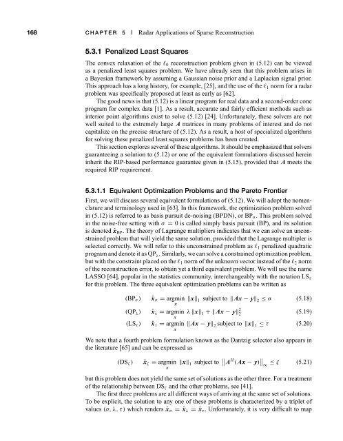
- Page 194 and 195: 5.3 SR Algorithms 169the value of o
- Page 196 and 197: 5.3 SR Algorithms 171takes special
- Page 198 and 199: 5.3 SR Algorithms 173The function f
- Page 200 and 201: 5.3 SR Algorithms 175of the TV norm
- Page 202 and 203: 5.3 SR Algorithms 177One can argue
- Page 204 and 205: 5.3 SR Algorithms 179probability ma
- Page 206 and 207: 5.3 SR Algorithms 181only a subset
- Page 208 and 209: 5.4 Sample Radar Applications 183pr
- Page 210 and 211: 5.4 Sample Radar Applications 185We
- Page 212 and 213: 5.4 Sample Radar Applications 187th
- Page 214 and 215: 5.4 Sample Radar Applications 189tu
- Page 216 and 217: 5.4 Sample Radar Applications 191Ra
- Page 218 and 219: 5.4 Sample Radar Applications 193Ta
- Page 221 and 222: 196 CHAPTER 5 Radar Applications of
- Page 223 and 224: 198 CHAPTER 5 Radar Applications of
- Page 225 and 226: 200 CHAPTER 5 Radar Applications of
- Page 227 and 228: 202 CHAPTER 5 Radar Applications of
- Page 229 and 230: 204 CHAPTER 5 Radar Applications of
- Page 231 and 232: 206 CHAPTER 5 Radar Applications of
- Page 233 and 234: 208 CHAPTER 5 Radar Applications of
- Page 236 and 237: Spotlight SyntheticAperture RadarCH
- Page 238 and 239: 6.1 Introduction 213• Image quali
- Page 240 and 241: 6.2 Mathematical Background 215andf
- Page 242 and 243:
6.2 Mathematical Background 2172π
- Page 245:
220 CHAPTER 6 Spotlight Synthetic A
- Page 249 and 250:
224 CHAPTER 6 Spotlight Synthetic A
- Page 251 and 252:
226 CHAPTER 6 Spotlight Synthetic A
- Page 253 and 254:
228 CHAPTER 6 Spotlight Synthetic A
- Page 256 and 257:
6.4 Sampling Requirements and Resol
- Page 258 and 259:
6.4 Sampling Requirements and Resol
- Page 261:
236 CHAPTER 6 Spotlight Synthetic A
- Page 264 and 265:
6.5 Image Reconstruction 239FIGURE
- Page 266 and 267:
6.6 Image Metrics 241The contrast r
- Page 268 and 269:
6.6 Image Metrics 243Along-track am
- Page 270:
6.7 Phase Error Effects 245TABLE 6-
- Page 273 and 274:
248 CHAPTER 6 Spotlight Synthetic A
- Page 275 and 276:
250 CHAPTER 6 Spotlight Synthetic A
- Page 277 and 278:
252 CHAPTER 6 Spotlight Synthetic A
- Page 279 and 280:
254 CHAPTER 6 Spotlight Synthetic A
- Page 281 and 282:
256 CHAPTER 6 Spotlight Synthetic A
- Page 283 and 284:
258 CHAPTER 6 Spotlight Synthetic A
- Page 285 and 286:
260 CHAPTER 7 Stripmap SAR3 m SAR O
- Page 287 and 288:
262 CHAPTER 7 Stripmap SAR• RMA i
- Page 289:
264 CHAPTER 7 Stripmap SARH 0 (ω)
- Page 293:
268 CHAPTER 7 Stripmap SARTABLE 7-1
- Page 299 and 300:
274 CHAPTER 7 Stripmap SARFIGURE 7-
- Page 301:
276 CHAPTER 7 Stripmap SAR−500Sce
- Page 310:
7.3 Doppler Beam Sharpening Extensi
- Page 313 and 314:
288 CHAPTER 7 Stripmap SARand in th
- Page 316 and 317:
7.4 Range-Doppler Algorithms 291to
- Page 318:
7.4 Range-Doppler Algorithms 293For
- Page 321:
296 CHAPTER 7 Stripmap SAR−150Col
- Page 325 and 326:
300 CHAPTER 7 Stripmap SAR33 cycles
- Page 327 and 328:
302 CHAPTER 7 Stripmap SARCrossrang
- Page 329:
304 CHAPTER 7 Stripmap SARfrom freq
- Page 332:
7.5 Range Migration Algorithm 307r,
- Page 335:
310 CHAPTER 7 Stripmap SARkx (rad/m
- Page 341:
316 CHAPTER 7 Stripmap SARThe diffe
- Page 345 and 346:
320 CHAPTER 7 Stripmap SARLet us re
- Page 347 and 348:
322 CHAPTER 7 Stripmap SARThe resul
- Page 349 and 350:
324 CHAPTER 7 Stripmap SARscene. Th
- Page 351 and 352:
326 CHAPTER 7 Stripmap SARdriven by
- Page 353 and 354:
328 CHAPTER 7 Stripmap SARTABLE 7-3
- Page 355 and 356:
330 CHAPTER 7 Stripmap SARFIGURE 7-
- Page 357 and 358:
332 CHAPTER 7 Stripmap SAR7.10 REFE
- Page 359 and 360:
334 CHAPTER 7 Stripmap SAR6. [MATLA
- Page 362 and 363:
Interferometric SAR andCoherent Exp
- Page 364 and 365:
8.1 Introduction 3398.1.1 Organizat
- Page 366 and 367:
8.1 Introduction 341Rsabnv rw x ,w
- Page 368 and 369:
8.2 Digital Terrain Models 343FIGUR
- Page 372 and 373:
8.3 Estimating Elevation Profiles U
- Page 374 and 375:
8.3 Estimating Elevation Profiles U
- Page 377:
352 CHAPTER 8 Interferometric SAR a
- Page 380:
8.3 Estimating Elevation Profiles U
- Page 383 and 384:
358 CHAPTER 8 Interferometric SAR a
- Page 387 and 388:
362 CHAPTER 8 Interferometric SAR a
- Page 390 and 391:
8.5 InSAR Processing Steps 365ξ ta
- Page 392:
8.5 InSAR Processing Steps 3670.1 0
- Page 395:
370 CHAPTER 8 Interferometric SAR a
- Page 398 and 399:
8.5 InSAR Processing Steps 373While
- Page 400 and 401:
8.6 Error Sources 375The second met
- Page 402 and 403:
8.6 Error Sources 377If sufficient
- Page 405 and 406:
380 CHAPTER 8 Interferometric SAR a
- Page 407 and 408:
382 CHAPTER 8 Interferometric SAR a
- Page 409 and 410:
384 CHAPTER 8 Interferometric SAR a
- Page 411 and 412:
386 CHAPTER 8 Interferometric SAR a
- Page 413:
388 CHAPTER 8 Interferometric SAR a
- Page 417 and 418:
392 CHAPTER 8 Interferometric SAR a
- Page 419 and 420:
394 CHAPTER 8 Interferometric SAR a
- Page 421 and 422:
396 CHAPTER 8 Interferometric SAR a
- Page 423 and 424:
398 CHAPTER 8 Interferometric SAR a
- Page 426 and 427:
Adaptive Digital BeamformingCHAPTER
- Page 428:
9.1 Introduction 403c k = clutter s
- Page 433 and 434:
408 CHAPTER 9 Adaptive Digital Beam
- Page 435 and 436:
410 CHAPTER 9 Adaptive Digital Beam
- Page 439:
414 CHAPTER 9 Adaptive Digital Beam
- Page 442 and 443:
9.2 Digital Beamforming Fundamental
- Page 445:
420 CHAPTER 9 Adaptive Digital Beam
- Page 448:
9.3 Adaptive Jammer Cancellation 42
- Page 451:
426 CHAPTER 9 Adaptive Digital Beam
- Page 454 and 455:
9.3 Adaptive Jammer Cancellation 42
- Page 456 and 457:
9.3 Adaptive Jammer Cancellation 43
- Page 458 and 459:
9.3 Adaptive Jammer Cancellation 43
- Page 467:
442 CHAPTER 9 Adaptive Digital Beam
- Page 472:
9.5 Wideband Cancellation 447FIGURE
- Page 475 and 476:
450 CHAPTER 9 Adaptive Digital Beam
- Page 477 and 478:
452 CHAPTER 9 Adaptive Digital Beam
- Page 479 and 480:
454 CHAPTER 10 Clutter Suppression
- Page 481 and 482:
456 CHAPTER 10 Clutter Suppression
- Page 483 and 484:
458 CHAPTER 10 Clutter Suppression
- Page 486 and 487:
10.2 Space-Time Signal Representati
- Page 488 and 489:
10.2 Space-Time Signal Representati
- Page 490 and 491:
10.2 Space-Time Signal Representati
- Page 492:
10.2 Space-Time Signal Representati
- Page 495 and 496:
470 CHAPTER 10 Clutter Suppression
- Page 497 and 498:
472 CHAPTER 10 Clutter Suppression
- Page 499 and 500:
474 CHAPTER 10 Clutter Suppression
- Page 501 and 502:
476 CHAPTER 10 Clutter Suppression
- Page 503 and 504:
478 CHAPTER 10 Clutter Suppression
- Page 506 and 507:
10.5 STAP Fundamentals 4810−5−1
- Page 508 and 509:
10.6 STAP Processing Architectures
- Page 510 and 511:
10.6 STAP Processing Architectures
- Page 512 and 513:
10.6 STAP Processing Architectures
- Page 514 and 515:
10.6 STAP Processing Architectures
- Page 516 and 517:
10.7 Other Considerations 4911 CPIM
- Page 518 and 519:
10.9 Summary 49310.7.3 Computationa
- Page 520 and 521:
10.10 References 495[12] Fenner, D.
- Page 522:
10.11 Problems 497the PSD in Figure
- Page 526 and 527:
11.2 Colored Space-Time Exploration
- Page 528 and 529:
11.2 Colored Space-Time Exploration
- Page 531 and 532:
506 CHAPTER 11 Space-Time Coding fo
- Page 537:
512 CHAPTER 11 Space-Time Coding fo
- Page 543 and 544:
518 CHAPTER 11 Space-Time Coding fo
- Page 545:
520 CHAPTER 11 Space-Time Coding fo
- Page 550 and 551:
11.8 References 525Cost reduction o
- Page 552:
11.9 Problems 52711.9.2 Equivalence
- Page 555 and 556:
530 CHAPTER 12 Electronic Protectio
- Page 557 and 558:
532 CHAPTER 12 Electronic Protectio
- Page 560:
12.2 Electronic Attack 535TABLE 12-
- Page 563:
538 CHAPTER 12 Electronic Protectio
- Page 566 and 567:
12.2 Electronic Attack 541variation
- Page 569 and 570:
544 CHAPTER 12 Electronic Protectio
- Page 571 and 572:
546 CHAPTER 12 Electronic Protectio
- Page 573 and 574:
548 CHAPTER 12 Electronic Protectio
- Page 575 and 576:
550 CHAPTER 12 Electronic Protectio
- Page 577 and 578:
552 CHAPTER 12 Electronic Protectio
- Page 579 and 580:
554 CHAPTER 12 Electronic Protectio
- Page 582 and 583:
12.5 Antenna-Based EP 557are adjust
- Page 586 and 587:
12.6 Transmitter-Based EP 561polari
- Page 589 and 590:
564 CHAPTER 12 Electronic Protectio
- Page 591 and 592:
566 CHAPTER 12 Electronic Protectio
- Page 593 and 594:
568 CHAPTER 12 Electronic Protectio
- Page 595 and 596:
570 CHAPTER 12 Electronic Protectio
- Page 597:
572 CHAPTER 12 Electronic Protectio
- Page 603 and 604:
578 CHAPTER 12 Electronic Protectio
- Page 605:
580 CHAPTER 12 Electronic Protectio
- Page 608 and 609:
12.11 Summary 583TABLE 12-4Summary
- Page 610:
12.14 Problems 585[9] Stimson, G.W.
- Page 614 and 615:
Introduction to RadarPolarimetryCHA
- Page 616 and 617:
13.1 Introduction 591and precipitat
- Page 618:
13.1 Introduction 593S: target scat
- Page 622 and 623:
13.2 Polarization 597After substitu
- Page 624 and 625:
13.2 Polarization 599zFIGURE 13-4Po
- Page 626 and 627:
13.3 Scattering Matrix 601left-hand
- Page 629 and 630:
604 CHAPTER 13 Introduction to Rada
- Page 631 and 632:
606 CHAPTER 13 Introduction to Rada
- Page 633 and 634:
608 CHAPTER 13 Introduction to Rada
- Page 635 and 636:
610 CHAPTER 13 Introduction to Rada
- Page 637:
612 CHAPTER 13 Introduction to Rada
- Page 640 and 641:
13.4 Radar Applications of Polarime
- Page 642 and 643:
13.4 Radar Applications of Polarime
- Page 644 and 645:
13.5 Measurement of the Scattering
- Page 646 and 647:
13.5 Measurement of the Scattering
- Page 648 and 649:
13.8 References 623• Lee, Jong-Se
- Page 650 and 651:
13.8 References 625[32] Kraus, J.D.
- Page 652:
13.9 Problems 627with the result in
- Page 656 and 657:
Automatic Target RecognitionCHAPTER
- Page 658 and 659:
14.2 Unified Framework for ATR 633P
- Page 660 and 661:
14.3 Metrics and Performance Predic
- Page 662 and 663:
14.3 Metrics and Performance Predic
- Page 664 and 665:
14.4 Synthetic Aperture Radar 639TA
- Page 666 and 667:
14.4 Synthetic Aperture Radar 641Te
- Page 668 and 669:
14.4 Synthetic Aperture Radar 64314
- Page 670 and 671:
14.4 Synthetic Aperture Radar 645Un
- Page 672 and 673:
14.4 Synthetic Aperture Radar 64714
- Page 674 and 675:
14.4 Synthetic Aperture Radar 649se
- Page 676 and 677:
14.4 Synthetic Aperture Radar 651th
- Page 678 and 679:
14.5 Inverse Synthetic Aperture Rad
- Page 680 and 681:
14.5 Inverse Synthetic Aperture Rad
- Page 682 and 683:
14.6 Passive Radar ATR 657radar sys
- Page 684 and 685:
14.7 High-Resolution Range Profiles
- Page 686 and 687:
14.9 Further Reading 661take a targ
- Page 688 and 689:
14.10 References 663[19] Q. H. Pham
- Page 690 and 691:
14.10 References 665[56] M. Martore
- Page 692 and 693:
14.10 References 667[92] E. Libby,
- Page 694 and 695:
Multitarget, MultisensorTrackingCHA
- Page 698 and 699:
15.1 Review Of Tracking Concepts 67
- Page 700:
15.1 Review Of Tracking Concepts 67
- Page 703 and 704:
678 CHAPTER 15 Multitarget, Multise
- Page 705 and 706:
680 CHAPTER 15 Multitarget, Multise
- Page 708 and 709:
15.2 Multitarget Tracking 683TABLE
- Page 710 and 711:
15.2 Multitarget Tracking 685remove
- Page 713 and 714:
688 CHAPTER 15 Multitarget, Multise
- Page 715 and 716:
690 CHAPTER 15 Multitarget, Multise
- Page 717:
692 CHAPTER 15 Multitarget, Multise
- Page 720 and 721:
15.5 Further Reading 69515.4 SUMMAR
- Page 722 and 723:
15.6 References 697[11] Blair, W.D.
- Page 724 and 725:
15.7 Problems 6992. Common metrics
- Page 726:
⎡⎤3 0 0 0 0 00 3 0 0 0 0P 2 =0
- Page 730 and 731:
Human Detection With Radar:Dismount
- Page 732 and 733:
environment that may mask the gener
- Page 734 and 735:
D s % = Boulic-Thalmann model param
- Page 736 and 737:
16.2 Characterizing the Human Radar
- Page 739 and 740:
714 CHAPTER 16 Human Detection With
- Page 741 and 742:
716 CHAPTER 16 Human Detection With
- Page 743 and 744:
718 CHAPTER 16 Human Detection With
- Page 745 and 746:
720 CHAPTER 16 Human Detection With
- Page 748 and 749:
16.4 Technical Challenges in Human
- Page 750 and 751:
16.4 Technical Challenges in Human
- Page 752 and 753:
16.5 Exploiting Knowledge for Detec
- Page 754 and 755:
16.7 Further Reading 729enable not
- Page 756 and 757:
16.8 References 731[13] Broggi, A.,
- Page 758 and 759:
16.8 References 733[53] G.E. Smith,
- Page 760 and 761:
16.8 References 735Conference on So
- Page 762:
16.9 Problems 737FIGURE 16-13Pendul
- Page 765:
740 CHAPTER 17 Advanced Processing
- Page 769 and 770:
744 CHAPTER 17 Advanced Processing
- Page 771 and 772:
746 CHAPTER 17 Advanced Processing
- Page 773 and 774:
748 CHAPTER 17 Advanced Processing
- Page 775 and 776:
750 CHAPTER 17 Advanced Processing
- Page 777 and 778:
752 CHAPTER 17 Advanced Processing
- Page 779 and 780:
754 CHAPTER 17 Advanced Processing
- Page 781 and 782:
756 CHAPTER 17 Advanced Processing
- Page 783 and 784:
758 CHAPTER 17 Advanced Processing
- Page 786 and 787:
17.3 Direct Signal and Multipath/Cl
- Page 788 and 789:
17.3 Direct Signal and Multipath/Cl
- Page 791 and 792:
766 CHAPTER 17 Advanced Processing
- Page 794 and 795:
17.4 Signal Processing Techniques f
- Page 796:
17.4 Signal Processing Techniques f
- Page 799 and 800:
774 CHAPTER 17 Advanced Processing
- Page 801 and 802:
776 CHAPTER 17 Advanced Processing
- Page 803 and 804:
778 CHAPTER 17 Advanced Processing
- Page 805 and 806:
780 CHAPTER 17 Advanced Processing
- Page 809:
784 CHAPTER 17 Advanced Processing
- Page 812:
17.5 2D-CCF Sidelobe Control 787TAB
- Page 816 and 817:
17.6 Multichannel Processing for De
- Page 819:
794 CHAPTER 17 Advanced Processing
- Page 822:
17.6 Multichannel Processing for De
- Page 828 and 829:
17.6 Multichannel Processing for De
- Page 830:
17.6 Multichannel Processing for De
- Page 835:
810 CHAPTER 17 Advanced Processing
- Page 838 and 839:
17.6 Multichannel Processing for De
- Page 840 and 841:
17.10 References 815While far from
- Page 842 and 843:
17.10 References 817[20] Chetty, K.
- Page 844 and 845:
17.11 Problems 819[52] Gao, Z., Tao
- Page 846:
17.11 Problems 8215. Using the sign
- Page 849 and 850:
824 Appendix A: Answers to Selected
- Page 851 and 852:
826 Appendix A: Answers to Selected
- Page 853:
828 Appendix A: Answers to Selected
- Page 857 and 858:
ResolutionResolution withDimension
- Page 859 and 860:
830 IndexASAR. See Advanced SAR (AS
- Page 861 and 862:
832 IndexCross-polarization (XPOL),
- Page 863 and 864:
834 IndexExciter-based EP (cont.)fr
- Page 865 and 866:
836 IndexInterferencecolored noise,
- Page 867 and 868:
838 IndexMoving target indication (
- Page 869 and 870:
840 IndexPOI. See Probability of in
- Page 871 and 872:
842 IndexSaturated (constant amplit
- Page 873 and 874:
844 IndexStripmap SAR (cont.)remote
- Page 875 and 876:
846 IndexWWald sequential test, com