- Page 2:
Principles of Modern Radar
- Page 5 and 6:
Published by SciTech Publishing, an
- Page 8:
Brief ContentsPreface xvPublisher A
- Page 11 and 12:
xContents3.6 Adaptive MIMO Radar 10
- Page 13 and 14:
xiiContents9.3 Adaptive Jammer Canc
- Page 15 and 16:
xivContents15.3 Multisensor Trackin
- Page 17 and 18:
xviPrefacehas always been the unlik
- Page 19 and 20:
Publisher AcknowledgmentsTechnical
- Page 21 and 22:
Editors and ContributorsVolume Edit
- Page 23 and 24:
xxiiEditors and ContributorsDr. Lis
- Page 25 and 26:
xxivEditors and ContributorsMr. Ara
- Page 27 and 28:
2 CHAPTER 1 Overview: Advanced Tech
- Page 30 and 31:
1.3 Radar and System Topologies 5FI
- Page 32 and 33:
1.4 Topics in Advanced Techniques 7
- Page 34 and 35:
1.4 Topics in Advanced Techniques 9
- Page 36 and 37:
1.4 Topics in Advanced Techniques 1
- Page 38 and 39:
1.4 Topics in Advanced Techniques 1
- Page 40 and 41:
1.6 References 15TABLE 1-1Summary o
- Page 42:
PART IWaveforms and SpectrumCHAPTER
- Page 45 and 46:
20 CHAPTER 2 Advanced Pulse Compres
- Page 47 and 48:
22 CHAPTER 2 Advanced Pulse Compres
- Page 49 and 50:
24 CHAPTER 2 Advanced Pulse Compres
- Page 51 and 52:
26 CHAPTER 2 Advanced Pulse Compres
- Page 53:
28 CHAPTER 2 Advanced Pulse Compres
- Page 60 and 61:
2.2 Stretch Processing 35is applied
- Page 62:
2.2 Stretch Processing 37TABLE 2-1
- Page 67 and 68:
42 CHAPTER 2 Advanced Pulse Compres
- Page 69:
44 CHAPTER 2 Advanced Pulse Compres
- Page 73:
48 CHAPTER 2 Advanced Pulse Compres
- Page 77 and 78:
52 CHAPTER 2 Advanced Pulse Compres
- Page 79 and 80:
54 CHAPTER 2 Advanced Pulse Compres
- Page 81 and 82:
56 CHAPTER 2 Advanced Pulse Compres
- Page 86 and 87:
2.5 Stepped Frequency Waveforms 61T
- Page 88:
2.5 Stepped Frequency Waveforms 63w
- Page 94 and 95:
2.5 Stepped Frequency Waveforms 69I
- Page 97:
72 CHAPTER 2 Advanced Pulse Compres
- Page 101:
76 CHAPTER 2 Advanced Pulse Compres
- Page 106 and 107:
2.9 References 812.7.4 SummaryWhile
- Page 108 and 109:
2.9 References 83[27] Taylor, Jr.,
- Page 110:
2.10 Problems 85shift across the pu
- Page 113:
88 CHAPTER 3 Optimal and Adaptive M
- Page 116 and 117:
3.2 Optimum MIMO Waveform Design fo
- Page 119 and 120:
94 CHAPTER 3 Optimal and Adaptive M
- Page 121 and 122:
96 CHAPTER 3 Optimal and Adaptive M
- Page 123 and 124:
98 CHAPTER 3 Optimal and Adaptive M
- Page 126 and 127:
3.4 Optimum MIMO Design for Target
- Page 128 and 129:
3.4 Optimum MIMO Design for Target
- Page 130:
3.5 Constrained Optimum MIMO Radar
- Page 133 and 134:
108 CHAPTER 3 Optimal and Adaptive
- Page 136:
3.6 Adaptive MIMO Radar 111SINR Los
- Page 140 and 141:
3.10 Problems 115[22] W. Y. Hsiang,
- Page 142:
3.10 Problems 1179. A constrained o
- Page 145:
120 CHAPTER 4 MIMO Radarperformance
- Page 148:
4.3 The MIMO Virtual Array 123separ
- Page 152 and 153:
4.4 MIMO Radar Signal Processing 12
- Page 154 and 155:
4.4 MIMO Radar Signal Processing 12
- Page 156 and 157:
4.4 MIMO Radar Signal Processing 13
- Page 159 and 160:
134 CHAPTER 4 MIMO RadarFIGURE 4-7T
- Page 161 and 162:
136 CHAPTER 4 MIMO Radar4.5.2 MIMO
- Page 163 and 164:
138 CHAPTER 4 MIMO Radarnamely, R
- Page 165 and 166:
140 CHAPTER 4 MIMO RadarTABLE 4-2 P
- Page 167 and 168:
142 CHAPTER 4 MIMO RadarSINR Loss (
- Page 169 and 170:
144 CHAPTER 4 MIMO Radar[10] H. V.
- Page 172 and 173:
Radar Applications of SparseReconst
- Page 174 and 175:
5.1 Introduction 149δ = M/N, the u
- Page 177 and 178:
152 CHAPTER 5 Radar Applications of
- Page 179 and 180:
154 CHAPTER 5 Radar Applications of
- Page 181 and 182:
156 CHAPTER 5 Radar Applications of
- Page 183 and 184:
158 CHAPTER 5 Radar Applications of
- Page 185 and 186:
160 CHAPTER 5 Radar Applications of
- Page 188 and 189:
5.2 CS Theory 163While the notion o
- Page 190 and 191:
5.2 CS Theory 165as , where is a b
- Page 192 and 193:
5.3 SR Algorithms 167than the norm
- Page 194 and 195:
5.3 SR Algorithms 169the value of o
- Page 196 and 197:
5.3 SR Algorithms 171takes special
- Page 198 and 199:
5.3 SR Algorithms 173The function f
- Page 200 and 201:
5.3 SR Algorithms 175of the TV norm
- Page 202 and 203:
5.3 SR Algorithms 177One can argue
- Page 204 and 205:
5.3 SR Algorithms 179probability ma
- Page 206 and 207:
5.3 SR Algorithms 181only a subset
- Page 208 and 209:
5.4 Sample Radar Applications 183pr
- Page 210 and 211:
5.4 Sample Radar Applications 185We
- Page 212 and 213:
5.4 Sample Radar Applications 187th
- Page 214 and 215:
5.4 Sample Radar Applications 189tu
- Page 216 and 217:
5.4 Sample Radar Applications 191Ra
- Page 218 and 219:
5.4 Sample Radar Applications 193Ta
- Page 221 and 222:
196 CHAPTER 5 Radar Applications of
- Page 223 and 224:
198 CHAPTER 5 Radar Applications of
- Page 225 and 226:
200 CHAPTER 5 Radar Applications of
- Page 227 and 228:
202 CHAPTER 5 Radar Applications of
- Page 229 and 230:
204 CHAPTER 5 Radar Applications of
- Page 231 and 232:
206 CHAPTER 5 Radar Applications of
- Page 233 and 234:
208 CHAPTER 5 Radar Applications of
- Page 236 and 237:
Spotlight SyntheticAperture RadarCH
- Page 238 and 239:
6.1 Introduction 213• Image quali
- Page 240 and 241:
6.2 Mathematical Background 215andf
- Page 242 and 243:
6.2 Mathematical Background 2172π
- Page 245:
220 CHAPTER 6 Spotlight Synthetic A
- Page 249 and 250:
224 CHAPTER 6 Spotlight Synthetic A
- Page 251 and 252:
226 CHAPTER 6 Spotlight Synthetic A
- Page 253 and 254:
228 CHAPTER 6 Spotlight Synthetic A
- Page 256 and 257:
6.4 Sampling Requirements and Resol
- Page 258 and 259:
6.4 Sampling Requirements and Resol
- Page 261:
236 CHAPTER 6 Spotlight Synthetic A
- Page 264 and 265:
6.5 Image Reconstruction 239FIGURE
- Page 266 and 267:
6.6 Image Metrics 241The contrast r
- Page 268 and 269:
6.6 Image Metrics 243Along-track am
- Page 270:
6.7 Phase Error Effects 245TABLE 6-
- Page 273 and 274:
248 CHAPTER 6 Spotlight Synthetic A
- Page 275 and 276:
250 CHAPTER 6 Spotlight Synthetic A
- Page 277 and 278:
252 CHAPTER 6 Spotlight Synthetic A
- Page 279 and 280:
254 CHAPTER 6 Spotlight Synthetic A
- Page 281 and 282:
256 CHAPTER 6 Spotlight Synthetic A
- Page 283 and 284:
258 CHAPTER 6 Spotlight Synthetic A
- Page 285 and 286:
260 CHAPTER 7 Stripmap SAR3 m SAR O
- Page 287 and 288:
262 CHAPTER 7 Stripmap SAR• RMA i
- Page 289:
264 CHAPTER 7 Stripmap SARH 0 (ω)
- Page 293:
268 CHAPTER 7 Stripmap SARTABLE 7-1
- Page 299 and 300:
274 CHAPTER 7 Stripmap SARFIGURE 7-
- Page 301:
276 CHAPTER 7 Stripmap SAR−500Sce
- Page 310:
7.3 Doppler Beam Sharpening Extensi
- Page 313 and 314:
288 CHAPTER 7 Stripmap SARand in th
- Page 316 and 317:
7.4 Range-Doppler Algorithms 291to
- Page 318:
7.4 Range-Doppler Algorithms 293For
- Page 321:
296 CHAPTER 7 Stripmap SAR−150Col
- Page 325 and 326:
300 CHAPTER 7 Stripmap SAR33 cycles
- Page 327 and 328:
302 CHAPTER 7 Stripmap SARCrossrang
- Page 329:
304 CHAPTER 7 Stripmap SARfrom freq
- Page 332:
7.5 Range Migration Algorithm 307r,
- Page 335:
310 CHAPTER 7 Stripmap SARkx (rad/m
- Page 341: 316 CHAPTER 7 Stripmap SARThe diffe
- Page 345 and 346: 320 CHAPTER 7 Stripmap SARLet us re
- Page 347 and 348: 322 CHAPTER 7 Stripmap SARThe resul
- Page 349 and 350: 324 CHAPTER 7 Stripmap SARscene. Th
- Page 351 and 352: 326 CHAPTER 7 Stripmap SARdriven by
- Page 353 and 354: 328 CHAPTER 7 Stripmap SARTABLE 7-3
- Page 355 and 356: 330 CHAPTER 7 Stripmap SARFIGURE 7-
- Page 357 and 358: 332 CHAPTER 7 Stripmap SAR7.10 REFE
- Page 359 and 360: 334 CHAPTER 7 Stripmap SAR6. [MATLA
- Page 362 and 363: Interferometric SAR andCoherent Exp
- Page 364 and 365: 8.1 Introduction 3398.1.1 Organizat
- Page 366 and 367: 8.1 Introduction 341Rsabnv rw x ,w
- Page 368 and 369: 8.2 Digital Terrain Models 343FIGUR
- Page 372 and 373: 8.3 Estimating Elevation Profiles U
- Page 374 and 375: 8.3 Estimating Elevation Profiles U
- Page 377: 352 CHAPTER 8 Interferometric SAR a
- Page 380: 8.3 Estimating Elevation Profiles U
- Page 383 and 384: 358 CHAPTER 8 Interferometric SAR a
- Page 387 and 388: 362 CHAPTER 8 Interferometric SAR a
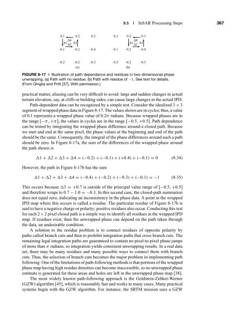
- Page 390 and 391: 8.5 InSAR Processing Steps 365ξ ta
- Page 394 and 395: 8.5 InSAR Processing Steps 369Along
- Page 397 and 398: 372 CHAPTER 8 Interferometric SAR a
- Page 399 and 400: 374 CHAPTER 8 Interferometric SAR a
- Page 401 and 402: 376 CHAPTER 8 Interferometric SAR a
- Page 403: 378 CHAPTER 8 Interferometric SAR a
- Page 406 and 407: 8.6 Error Sources 381Equations (8.4
- Page 408 and 409: TABLE 8-3 Approximate Parameters of
- Page 410 and 411: 8.7 Some Notable InSAR Systems 385(
- Page 412 and 413: 8.8 Other Coherent Exploitation Tec
- Page 415: 390 CHAPTER 8 Interferometric SAR a
- Page 418 and 419: 8.11 References 3938.11 REFERENCES[
- Page 420 and 421: 8.11 References 395[38] Zebker, H.A
- Page 422 and 423: 8.12 Problems 397[74] Romeiser, R.
- Page 424: PART IIIArray Processing and Interf
- Page 427 and 428: 402 CHAPTER 9 Adaptive Digital Beam
- Page 430: 9.2 Digital Beamforming Fundamental
- Page 434 and 435: 9.2 Digital Beamforming Fundamental
- Page 436: 9.2 Digital Beamforming Fundamental
- Page 441 and 442: 416 CHAPTER 9 Adaptive Digital Beam
- Page 443:
418 CHAPTER 9 Adaptive Digital Beam
- Page 447 and 448:
422 CHAPTER 9 Adaptive Digital Beam
- Page 450 and 451:
9.3 Adaptive Jammer Cancellation 42
- Page 453 and 454:
428 CHAPTER 9 Adaptive Digital Beam
- Page 455 and 456:
430 CHAPTER 9 Adaptive Digital Beam
- Page 457 and 458:
432 CHAPTER 9 Adaptive Digital Beam
- Page 459:
434 CHAPTER 9 Adaptive Digital Beam
- Page 470:
9.5 Wideband Cancellation 445where
- Page 474 and 475:
9.8 References 449the length of the
- Page 476 and 477:
9.9 Problems 451[32] Golub, G.H. an
- Page 478 and 479:
Clutter Suppression UsingSpace-Time
- Page 480 and 481:
10.1 Introduction 455It is known th
- Page 482 and 483:
10.1 Introduction 457where [w] ∗
- Page 484:
10.2 Space-Time Signal Representati
- Page 487 and 488:
462 CHAPTER 10 Clutter Suppression
- Page 489 and 490:
464 CHAPTER 10 Clutter Suppression
- Page 491 and 492:
466 CHAPTER 10 Clutter Suppression
- Page 494 and 495:
10.2 Space-Time Signal Representati
- Page 496 and 497:
10.2 Space-Time Signal Representati
- Page 498 and 499:
10.3 Space-Time Properties of Groun
- Page 500 and 501:
10.4 Space-Time Processing 475X k =
- Page 502 and 503:
10.4 Space-Time Processing 477Proba
- Page 504:
10.5 STAP Fundamentals 479It is con
- Page 507 and 508:
482 CHAPTER 10 Clutter Suppression
- Page 509 and 510:
484 CHAPTER 10 Clutter Suppression
- Page 511 and 512:
486 CHAPTER 10 Clutter Suppression
- Page 513 and 514:
488 CHAPTER 10 Clutter Suppression
- Page 515 and 516:
490 CHAPTER 10 Clutter Suppression
- Page 517 and 518:
492 CHAPTER 10 Clutter Suppression
- Page 519 and 520:
494 CHAPTER 10 Clutter Suppression
- Page 521 and 522:
496 CHAPTER 10 Clutter Suppression
- Page 524:
Space-Time Coding for ActiveAntenna
- Page 527 and 528:
502 CHAPTER 11 Space-Time Coding fo
- Page 529:
504 CHAPTER 11 Space-Time Coding fo
- Page 532:
11.2 Colored Space-Time Exploration
- Page 540:
11.3 Interleaved Scanning (Slow-Tim
- Page 544 and 545:
11.4 Code Selection and Grating Lob
- Page 549 and 550:
524 CHAPTER 11 Space-Time Coding fo
- Page 551 and 552:
526 CHAPTER 11 Space-Time Coding fo
- Page 554 and 555:
CHAPTERElectronic Protection12Aram
- Page 556 and 557:
12.1 Introduction 531c speed of lig
- Page 558:
12.2 Electronic Attack 533PRIPWRBMR
- Page 562 and 563:
12.2 Electronic Attack 537figure in
- Page 565 and 566:
540 CHAPTER 12 Electronic Protectio
- Page 567:
542 CHAPTER 12 Electronic Protectio
- Page 570 and 571:
12.3 EW-Related Formulas 545provide
- Page 572 and 573:
12.3 EW-Related Formulas 547incur t
- Page 574 and 575:
12.3 EW-Related Formulas 549−40.0
- Page 576 and 577:
12.3 EW-Related Formulas 551Section
- Page 578 and 579:
12.4 EP Overview 553100FIGURE 12-8J
- Page 580:
12.5 Antenna-Based EP 55512.5.1 Low
- Page 583:
558 CHAPTER 12 Electronic Protectio
- Page 587:
562 CHAPTER 12 Electronic Protectio
- Page 590 and 591:
12.7 Exciter-Based EP 565erstwhile
- Page 592 and 593:
12.8 Receiver-Based EP 567RSN bandw
- Page 594 and 595:
12.8 Receiver-Based EP 56912.8.3 Wi
- Page 596 and 597:
12.8 Receiver-Based EP 571to the de
- Page 599:
574 CHAPTER 12 Electronic Protectio
- Page 604 and 605:
12.10 Data Processor-Based EP 579Th
- Page 607 and 608:
582 CHAPTER 12 Electronic Protectio
- Page 609 and 610:
584 CHAPTER 12 Electronic Protectio
- Page 612:
PART IVPost-Processing Consideratio
- Page 615 and 616:
590 CHAPTER 13 Introduction to Rada
- Page 617 and 618:
592 CHAPTER 13 Introduction to Rada
- Page 620:
13.2 Polarization 595Therefore, we
- Page 623 and 624:
598 CHAPTER 13 Introduction to Rada
- Page 625 and 626:
600 CHAPTER 13 Introduction to Rada
- Page 627:
602 CHAPTER 13 Introduction to Rada
- Page 630 and 631:
13.3 Scattering Matrix 605in (13.34
- Page 632 and 633:
13.3 Scattering Matrix 607polarizat
- Page 634 and 635:
13.3 Scattering Matrix 609G ψ = G
- Page 636 and 637:
13.4 Radar Applications of Polarime
- Page 639 and 640:
614 CHAPTER 13 Introduction to Rada
- Page 641 and 642:
616 CHAPTER 13 Introduction to Rada
- Page 643 and 644:
618 CHAPTER 13 Introduction to Rada
- Page 645 and 646:
620 CHAPTER 13 Introduction to Rada
- Page 647 and 648:
622 CHAPTER 13 Introduction to Rada
- Page 649 and 650:
624 CHAPTER 13 Introduction to Rada
- Page 651 and 652:
626 CHAPTER 13 Introduction to Rada
- Page 654:
13.9 Problems 62915. A left-circula
- Page 657 and 658:
632 CHAPTER 14 Automatic Target Rec
- Page 659 and 660:
634 CHAPTER 14 Automatic Target Rec
- Page 661 and 662:
636 CHAPTER 14 Automatic Target Rec
- Page 663 and 664:
638 CHAPTER 14 Automatic Target Rec
- Page 665 and 666:
640 CHAPTER 14 Automatic Target Rec
- Page 667 and 668:
642 CHAPTER 14 Automatic Target Rec
- Page 669 and 670:
644 CHAPTER 14 Automatic Target Rec
- Page 671 and 672:
646 CHAPTER 14 Automatic Target Rec
- Page 673 and 674:
648 CHAPTER 14 Automatic Target Rec
- Page 675 and 676:
650 CHAPTER 14 Automatic Target Rec
- Page 677 and 678:
652 CHAPTER 14 Automatic Target Rec
- Page 679 and 680:
654 CHAPTER 14 Automatic Target Rec
- Page 681 and 682:
656 CHAPTER 14 Automatic Target Rec
- Page 683 and 684:
658 CHAPTER 14 Automatic Target Rec
- Page 685 and 686:
660 CHAPTER 14 Automatic Target Rec
- Page 687 and 688:
662 CHAPTER 14 Automatic Target Rec
- Page 689 and 690:
664 CHAPTER 14 Automatic Target Rec
- Page 691 and 692:
666 CHAPTER 14 Automatic Target Rec
- Page 693 and 694:
668 CHAPTER 14 Automatic Target Rec
- Page 695:
670 CHAPTER 15 Multitarget, Multise
- Page 699 and 700:
674 CHAPTER 15 Multitarget, Multise
- Page 702 and 703:
15.2 Multitarget Tracking 677state
- Page 704 and 705:
15.2 Multitarget Tracking 679track
- Page 706:
15.2 Multitarget Tracking 681Probab
- Page 709 and 710:
684 CHAPTER 15 Multitarget, Multise
- Page 711:
686 CHAPTER 15 Multitarget, Multise
- Page 714 and 715:
15.2 Multitarget Tracking 689Mode 1
- Page 716 and 717:
15.3 Multisensor Tracking 69115.3 M
- Page 719 and 720:
694 CHAPTER 15 Multitarget, Multise
- Page 721 and 722:
696 CHAPTER 15 Multitarget, Multise
- Page 723 and 724:
698 CHAPTER 15 Multitarget, Multise
- Page 725 and 726:
700 CHAPTER 15 Multitarget, Multise
- Page 728:
PART VEmerging TechniquesCHAPTER 16
- Page 731 and 732:
706 CHAPTER 16 Human Detection With
- Page 733 and 734:
708 CHAPTER 16 Human Detection With
- Page 735 and 736:
710 CHAPTER 16 Human Detection With
- Page 737:
712 CHAPTER 16 Human Detection With
- Page 740 and 741:
16.2 Characterizing the Human Radar
- Page 742 and 743:
16.2 Characterizing the Human Radar
- Page 744 and 745:
16.3 Spectrogram Analysis of Human
- Page 746:
16.3 Spectrogram Analysis of Human
- Page 749 and 750:
724 CHAPTER 16 Human Detection With
- Page 751 and 752:
726 CHAPTER 16 Human Detection With
- Page 753 and 754:
728 CHAPTER 16 Human Detection With
- Page 755 and 756:
730 CHAPTER 16 Human Detection With
- Page 757 and 758:
732 CHAPTER 16 Human Detection With
- Page 759 and 760:
734 CHAPTER 16 Human Detection With
- Page 761 and 762:
736 CHAPTER 16 Human Detection With
- Page 764 and 765:
Advanced Processing Methodsfor Pass
- Page 768 and 769:
17.1 Introduction 743to the usual c
- Page 770 and 771:
c = velocity of propagation (speed
- Page 772 and 773:
17.2 Evaluation of the 2D-CCF for t
- Page 774 and 775:
17.2 Evaluation of the 2D-CCF for t
- Page 776 and 777:
17.2 Evaluation of the 2D-CCF for t
- Page 778 and 779:
17.2 Evaluation of the 2D-CCF for t
- Page 780 and 781:
17.3 Direct Signal and Multipath/Cl
- Page 782 and 783:
17.3 Direct Signal and Multipath/Cl
- Page 784:
17.3 Direct Signal and Multipath/Cl
- Page 787 and 788:
762 CHAPTER 17 Advanced Processing
- Page 789:
764 CHAPTER 17 Advanced Processing
- Page 792:
17.4 Signal Processing Techniques f
- Page 795 and 796:
770 CHAPTER 17 Advanced Processing
- Page 798 and 799:
17.4 Signal Processing Techniques f
- Page 800 and 801:
17.5 2D-CCF Sidelobe Control 775sup
- Page 802 and 803:
17.5 2D-CCF Sidelobe Control 777Aut
- Page 804 and 805:
17.5 2D-CCF Sidelobe Control 779hig
- Page 806:
17.5 2D-CCF Sidelobe Control 781Acc
- Page 811 and 812:
786 CHAPTER 17 Advanced Processing
- Page 814:
17.5 2D-CCF Sidelobe Control 789REF
- Page 817:
792 CHAPTER 17 Advanced Processing
- Page 821 and 822:
796 CHAPTER 17 Advanced Processing
- Page 825:
800 CHAPTER 17 Advanced Processing
- Page 829 and 830:
804 CHAPTER 17 Advanced Processing
- Page 834 and 835:
17.6 Multichannel Processing for De
- Page 837 and 838:
812 CHAPTER 17 Advanced Processing
- Page 839 and 840:
814 CHAPTER 17 Advanced Processing
- Page 841 and 842:
816 CHAPTER 17 Advanced Processing
- Page 843 and 844:
818 CHAPTER 17 Advanced Processing
- Page 845 and 846:
820 CHAPTER 17 Advanced Processing
- Page 848 and 849:
Appendix A: Answers toSelected Prob
- Page 850 and 851:
Chapter 71. Waveform bandwidth = 15
- Page 852 and 853:
Appendix A: Answers to Selected Pro
- Page 856 and 857:
Signal Analysis and ProcessingSelec
- Page 858 and 859:
IndexNote: Page numbers followed by
- Page 860 and 861:
Index 831Channel matrix, MIMO, 125-
- Page 862 and 863:
Index 833notes on, 285RMC. See Rang
- Page 864 and 865:
Index 835SINR loss for, 141, 142fGr
- Page 866 and 867:
Index 837Layover and foreshortening
- Page 868 and 869:
Index 839design approaches, 51-52Do
- Page 870 and 871:
Index 841preselection, 567-568spati
- Page 872 and 873:
Index 843computational demands, 493
- Page 874 and 875:
Index 845TED. See Total energy dete
- Page 876:
Principles of Modern Radar: Advance