- Page 2:
This page intentionally left blank
- Page 6:
Physicists. He is also a Director o
- Page 10:
cambridge university pressCambridge
- Page 14:
CONTENTS2.2 Integration 59Integrati
- Page 18:
CONTENTS7.7 Equations of lines, pla
- Page 22:
CONTENTS12.2 The Fourier coefficien
- Page 26:
CONTENTS18.6 Spherical Bessel funct
- Page 30:
CONTENTS24.9 Cauchy’s theorem 849
- Page 34:
CONTENTS29.6 Characters 1092Orthogo
- Page 40:
CONTENTSI am the very Model for a S
- Page 44:
PREFACE TO THE THIRD EDITIONthe phy
- Page 48:
Preface to the second editionSince
- Page 52:
Preface to the first editionA knowl
- Page 56:
PREFACE TO THE FIRST EDITIONsupport
- Page 62:
PRELIMINARY ALGEBRAforms an equatio
- Page 66:
PRELIMINARY ALGEBRAmany real roots
- Page 70:
PRELIMINARY ALGEBRAat a value of x
- Page 74:
PRELIMINARY ALGEBRAwhere f 1 (x) is
- Page 78:
PRELIMINARY ALGEBRAIn the case of a
- Page 82:
PRELIMINARY ALGEBRAdrawn through R,
- Page 86:
PRELIMINARY ALGEBRAand use made of
- Page 90:
PRELIMINARY ALGEBRAwith the coordin
- Page 94:
PRELIMINARY ALGEBRAthe well-known r
- Page 98:
PRELIMINARY ALGEBRAnumerators on bo
- Page 102:
PRELIMINARY ALGEBRAWe illustrate th
- Page 106:
PRELIMINARY ALGEBRAIn this form, al
- Page 110:
PRELIMINARY ALGEBRAIn fact, the gen
- Page 114:
PRELIMINARY ALGEBRAThe first is a f
- Page 118:
PRELIMINARY ALGEBRAbe obvious, but
- Page 122:
PRELIMINARY ALGEBRAThis is precisel
- Page 126:
PRELIMINARY ALGEBRA◮The prime int
- Page 130:
PRELIMINARY ALGEBRA1.8 ExercisesPol
- Page 134:
PRELIMINARY ALGEBRA1.16 Express the
- Page 138:
PRELIMINARY ALGEBRA1.11 Show that t
- Page 142:
PRELIMINARY CALCULUSf(x +∆x)AP∆
- Page 146:
PRELIMINARY CALCULUS◮Find from fi
- Page 150:
PRELIMINARY CALCULUSand using (2.6)
- Page 154:
PRELIMINARY CALCULUS◮Find dy/dx i
- Page 158:
PRELIMINARY CALCULUSf(x)QABCSFigure
- Page 162:
PRELIMINARY CALCULUSf(x)GxFigure 2.
- Page 166:
PRELIMINARY CALCULUSrelative to the
- Page 170:
PRELIMINARY CALCULUSf(x)a b cxFigur
- Page 174:
PRELIMINARY CALCULUSIn each case, a
- Page 178:
PRELIMINARY CALCULUSf(x)ax 1 x 2 x
- Page 182:
PRELIMINARY CALCULUSFrom the last t
- Page 186:
PRELIMINARY CALCULUS◮Evaluate the
- Page 190:
PRELIMINARY CALCULUSSincethe requir
- Page 194:
PRELIMINARY CALCULUSThe separation
- Page 198:
PRELIMINARY CALCULUS2.2.10 Infinite
- Page 202:
PRELIMINARY CALCULUS2.2.12 Integral
- Page 206:
PRELIMINARY CALCULUSf(x)y = f(x)∆
- Page 210:
PRELIMINARY CALCULUS◮Find the vol
- Page 214:
PRELIMINARY CALCULUSOcCρr +∆rrρ
- Page 218:
PRELIMINARY CALCULUS(c) [(x − a)/
- Page 222:
PRELIMINARY CALCULUSy2aπa2πaxFigu
- Page 226:
COMPLEX NUMBERS AND HYPERBOLIC FUNC
- Page 230:
COMPLEX NUMBERS AND HYPERBOLIC FUNC
- Page 234:
COMPLEX NUMBERS AND HYPERBOLIC FUNC
- Page 238:
COMPLEX NUMBERS AND HYPERBOLIC FUNC
- Page 242:
COMPLEX NUMBERS AND HYPERBOLIC FUNC
- Page 246:
COMPLEX NUMBERS AND HYPERBOLIC FUNC
- Page 250:
COMPLEX NUMBERS AND HYPERBOLIC FUNC
- Page 254:
COMPLEX NUMBERS AND HYPERBOLIC FUNC
- Page 258:
COMPLEX NUMBERS AND HYPERBOLIC FUNC
- Page 262:
COMPLEX NUMBERS AND HYPERBOLIC FUNC
- Page 266:
COMPLEX NUMBERS AND HYPERBOLIC FUNC
- Page 270:
COMPLEX NUMBERS AND HYPERBOLIC FUNC
- Page 274:
COMPLEX NUMBERS AND HYPERBOLIC FUNC
- Page 278:
COMPLEX NUMBERS AND HYPERBOLIC FUNC
- Page 282:
COMPLEX NUMBERS AND HYPERBOLIC FUNC
- Page 286:
COMPLEX NUMBERS AND HYPERBOLIC FUNC
- Page 290:
SERIES AND LIMITSsome sort of relat
- Page 294:
SERIES AND LIMITSFor a series with
- Page 298:
SERIES AND LIMITSThe difference met
- Page 302:
SERIES AND LIMITS◮Sum the seriesN
- Page 306:
SERIES AND LIMITSAgain using the Ma
- Page 310:
SERIES AND LIMITSwhich is merely th
- Page 314:
SERIES AND LIMITS◮Given that the
- Page 318:
SERIES AND LIMITSThe divergence of
- Page 322:
SERIES AND LIMITSalthough in princi
- Page 326:
SERIES AND LIMITSr = − exp iθ. T
- Page 330:
SERIES AND LIMITS4.6 Taylor seriesT
- Page 334:
SERIES AND LIMITSx = a + h in the a
- Page 338:
SERIES AND LIMITSvalue of ξ that s
- Page 342:
SERIES AND LIMITS◮Evaluate the li
- Page 346:
SERIES AND LIMITSSummary of methods
- Page 350:
SERIES AND LIMITS4.15 Prove that∞
- Page 354:
SERIES AND LIMITSsin 3x(a) limx→0
- Page 358:
SERIES AND LIMITS4.15 Divide the se
- Page 362:
PARTIAL DIFFERENTIATIONto x and y r
- Page 366:
PARTIAL DIFFERENTIATIONcan be obtai
- Page 370:
PARTIAL DIFFERENTIATIONit exact. Co
- Page 374:
PARTIAL DIFFERENTIATIONFrom equatio
- Page 378:
PARTIAL DIFFERENTIATIONThus, from (
- Page 382:
PARTIAL DIFFERENTIATIONtheorem then
- Page 386:
PARTIAL DIFFERENTIATIONTo establish
- Page 390:
PARTIAL DIFFERENTIATIONmaximum0.40.
- Page 394:
PARTIAL DIFFERENTIATIONvaried. Howe
- Page 398:
PARTIAL DIFFERENTIATION◮Find the
- Page 402:
PARTIAL DIFFERENTIATION◮A system
- Page 406:
PARTIAL DIFFERENTIATIONP 1PP 2yf(x,
- Page 410:
PARTIAL DIFFERENTIATION5.11 Thermod
- Page 414:
PARTIAL DIFFERENTIATIONAlthough the
- Page 418:
PARTIAL DIFFERENTIATION(a) Find all
- Page 422:
PARTIAL DIFFERENTIATIONthe horizont
- Page 426:
PARTIAL DIFFERENTIATIONBy consideri
- Page 430:
PARTIAL DIFFERENTIATION5.19 The cos
- Page 434:
MULTIPLE INTEGRALSydSdxdA = dxdyRVd
- Page 438:
MULTIPLE INTEGRALSy1dyRx + y =100dx
- Page 442:
MULTIPLE INTEGRALSzcdV = dx dy dzdz
- Page 446:
MULTIPLE INTEGRALSzz =2yz = x 2 + y
- Page 450:
MULTIPLE INTEGRALSza√a2 − z 2dz
- Page 454:
MULTIPLE INTEGRALSaθdCFigure 6.8Su
- Page 458:
MULTIPLE INTEGRALSyu =constantv =co
- Page 462:
MULTIPLE INTEGRALS◮Evaluate the d
- Page 466:
MULTIPLE INTEGRALSzRTu = c 1v = c 2
- Page 470:
MULTIPLE INTEGRALSwhich agrees with
- Page 474:
MULTIPLE INTEGRALS6.6 The function(
- Page 478:
MULTIPLE INTEGRALSover the ellipsoi
- Page 482:
7Vector algebraThis chapter introdu
- Page 486:
VECTOR ALGEBRAabcb + cbcab + ca +(b
- Page 490:
VECTOR ALGEBRACEAGFDacBbOFigure 7.6
- Page 494:
VECTOR ALGEBRAkaja z ka y ja x iiFi
- Page 498:
VECTOR ALGEBRAFrom (7.15) we see th
- Page 502:
VECTOR ALGEBRAa × bθbaFigure 7.9s
- Page 506:
VECTOR ALGEBRAis the forward direct
- Page 510:
VECTOR ALGEBRA◮Find the volume V
- Page 514:
VECTOR ALGEBRAˆnARadrOFigure 7.13
- Page 518:
VECTOR ALGEBRAPp − apdAbθaOFigur
- Page 522:
VECTOR ALGEBRAQbqˆnPpaOFigure 7.16
- Page 526:
VECTOR ALGEBRAnot coplanar. Moreove
- Page 530:
VECTOR ALGEBRA7.12 The plane P 1 co
- Page 534:
VECTOR ALGEBRA7.22 In subsection 7.
- Page 538:
VECTOR ALGEBRAof vector plots for p
- Page 542:
MATRICES AND VECTOR SPACESa discuss
- Page 546:
MATRICES AND VECTOR SPACESWe reiter
- Page 550:
MATRICES AND VECTOR SPACES8.1.3 Som
- Page 554:
MATRICES AND VECTOR SPACESmay be th
- Page 558:
MATRICES AND VECTOR SPACESIn a simi
- Page 562:
MATRICES AND VECTOR SPACES◮The ma
- Page 566:
MATRICES AND VECTOR SPACESThese are
- Page 570:
MATRICES AND VECTOR SPACES◮Find t
- Page 574:
MATRICES AND VECTOR SPACESthe right
- Page 578:
MATRICES AND VECTOR SPACESdetermina
- Page 582:
MATRICES AND VECTOR SPACESIt follow
- Page 586:
MATRICES AND VECTOR SPACESequivalen
- Page 590:
MATRICES AND VECTOR SPACESand may b
- Page 594:
MATRICES AND VECTOR SPACESmay be sh
- Page 598:
MATRICES AND VECTOR SPACESClearly r
- Page 602:
MATRICES AND VECTOR SPACESHence 〈
- Page 606:
MATRICES AND VECTOR SPACESWe also s
- Page 610:
MATRICES AND VECTOR SPACESa result
- Page 614:
MATRICES AND VECTOR SPACESHence λ
- Page 618:
MATRICES AND VECTOR SPACES8.14 Dete
- Page 622:
MATRICES AND VECTOR SPACES◮Constr
- Page 626:
MATRICES AND VECTOR SPACESComparing
- Page 630:
MATRICES AND VECTOR SPACESthat is,
- Page 634:
MATRICES AND VECTOR SPACES| exp A|.
- Page 638:
MATRICES AND VECTOR SPACESalso. Ano
- Page 642:
MATRICES AND VECTOR SPACES8.17.2 Qu
- Page 646:
MATRICES AND VECTOR SPACESIf a vect
- Page 650:
MATRICES AND VECTOR SPACES◮Show t
- Page 654:
MATRICES AND VECTOR SPACESThis set
- Page 658:
MATRICES AND VECTOR SPACESthe uniqu
- Page 662:
MATRICES AND VECTOR SPACESthe numbe
- Page 666:
MATRICES AND VECTOR SPACESnon-zero
- Page 670:
MATRICES AND VECTOR SPACESUsing the
- Page 674:
MATRICES AND VECTOR SPACES8.3 Using
- Page 678:
MATRICES AND VECTOR SPACES(b) find
- Page 682:
MATRICES AND VECTOR SPACES8.26 Show
- Page 686:
MATRICES AND VECTOR SPACES8.40 Find
- Page 690:
9Normal modesAny student of the phy
- Page 694:
NORMAL MODESP P Pθ 1θ 2θ 2lθ 1
- Page 698:
NORMAL MODESfrequency corresponds t
- Page 702:
NORMAL MODESThe final and most comp
- Page 706:
NORMAL MODESThe potential matrix is
- Page 710:
NORMAL MODESneous equations for α
- Page 714:
NORMAL MODESbe shown that they do p
- Page 718:
NORMAL MODESunder gravity. At time
- Page 722:
NORMAL MODES9.8 (It is recommended
- Page 726:
10Vector calculusIn chapter 7 we di
- Page 730:
VECTOR CALCULUSyê φjê ρρiφxFi
- Page 734:
VECTOR CALCULUSThe order of the fac
- Page 738:
VECTOR CALCULUSzCˆnPˆtˆbr(u)OyxF
- Page 742:
VECTOR CALCULUSTherefore, rememberi
- Page 746:
VECTOR CALCULUSFinally, we note tha
- Page 750:
VECTOR CALCULUStotal derivative, th
- Page 754:
VECTOR CALCULUSmathematical point o
- Page 758:
VECTOR CALCULUS◮For the function
- Page 762:
VECTOR CALCULUSIn addition to these
- Page 766:
VECTOR CALCULUS∇(φ + ψ) =∇φ
- Page 770:
VECTOR CALCULUSa is a vector field,
- Page 774:
VECTOR CALCULUSρ, φ, z, wherex =
- Page 778:
VECTOR CALCULUS∇Φ = ∂Φ∂ρ
- Page 782:
VECTOR CALCULUSand r ≥ 0, 0 ≤
- Page 786:
VECTOR CALCULUS10.10 General curvil
- Page 790:
VECTOR CALCULUSFor orthogonal coord
- Page 794:
VECTOR CALCULUS◮Prove the express
- Page 798:
VECTOR CALCULUS10.3 The general equ
- Page 802:
VECTOR CALCULUSUse this formula to
- Page 806:
VECTOR CALCULUS10.21 Paraboloidal c
- Page 810:
VECTOR CALCULUS10.23 The tangent ve
- Page 814:
LINE, SURFACE AND VOLUME INTEGRALSE
- Page 818:
LINE, SURFACE AND VOLUME INTEGRALSy
- Page 822:
LINE, SURFACE AND VOLUME INTEGRALSi
- Page 826:
LINE, SURFACE AND VOLUME INTEGRALSy
- Page 830:
LINE, SURFACE AND VOLUME INTEGRALSy
- Page 834:
LINE, SURFACE AND VOLUME INTEGRALSw
- Page 838:
LINE, SURFACE AND VOLUME INTEGRALSS
- Page 842:
LINE, SURFACE AND VOLUME INTEGRALSw
- Page 846:
LINE, SURFACE AND VOLUME INTEGRALSd
- Page 850:
LINE, SURFACE AND VOLUME INTEGRALSI
- Page 854:
LINE, SURFACE AND VOLUME INTEGRALS1
- Page 858:
LINE, SURFACE AND VOLUME INTEGRALSz
- Page 862:
LINE, SURFACE AND VOLUME INTEGRALSy
- Page 866:
LINE, SURFACE AND VOLUME INTEGRALS1
- Page 870:
LINE, SURFACE AND VOLUME INTEGRALS1
- Page 874:
LINE, SURFACE AND VOLUME INTEGRALSS
- Page 878:
LINE, SURFACE AND VOLUME INTEGRALSi
- Page 882:
LINE, SURFACE AND VOLUME INTEGRALS1
- Page 886:
LINE, SURFACE AND VOLUME INTEGRALS1
- Page 890:
FOURIER SERIESf(x)xLLFigure 12.1 An
- Page 894:
FOURIER SERIESapply for r = 0 as we
- Page 898:
FOURIER SERIESare not used as often
- Page 902:
FOURIER SERIES(a)0L(b)0L2L(c)0L2L(d
- Page 906:
FOURIER SERIESconverge to the corre
- Page 910:
FOURIER SERIES12.8 Parseval’s the
- Page 914:
FOURIER SERIESbe better for numeric
- Page 918:
FOURIER SERIES12.21 Find the comple
- Page 922:
FOURIER SERIES12.21 c n =[(−1) n
- Page 926:
INTEGRAL TRANSFORMSc(ω)expiωt−
- Page 930:
INTEGRAL TRANSFORMS◮Find the Four
- Page 934:
INTEGRAL TRANSFORMSYyk ′k0θx−Y
- Page 938:
INTEGRAL TRANSFORMSequals zero. Thi
- Page 942:
INTEGRAL TRANSFORMS◮Prove relatio
- Page 946:
INTEGRAL TRANSFORMS(i) Differentiat
- Page 950:
INTEGRAL TRANSFORMSg(y)(a)(b)(c)(d)
- Page 954:
INTEGRAL TRANSFORMSgiven by∫1 ∞
- Page 958:
INTEGRAL TRANSFORMS◮Prove the Wie
- Page 962:
INTEGRAL TRANSFORMStwo- or three-di
- Page 966:
INTEGRAL TRANSFORMS(iii) Once again
- Page 970:
INTEGRAL TRANSFORMS◮Find the Lapl
- Page 974:
INTEGRAL TRANSFORMSFigure 13.7text)
- Page 978:
INTEGRAL TRANSFORMS13.4 Exercises13
- Page 982:
INTEGRAL TRANSFORMS13.10 In many ap
- Page 986:
INTEGRAL TRANSFORMS13.18 The equiva
- Page 990:
INTEGRAL TRANSFORMS13.27 The functi
- Page 994:
14First-order ordinary differential
- Page 998:
FIRST-ORDER ORDINARY DIFFERENTIAL E
- Page 1002:
FIRST-ORDER ORDINARY DIFFERENTIAL E
- Page 1006:
FIRST-ORDER ORDINARY DIFFERENTIAL E
- Page 1010:
FIRST-ORDER ORDINARY DIFFERENTIAL E
- Page 1014:
FIRST-ORDER ORDINARY DIFFERENTIAL E
- Page 1018:
FIRST-ORDER ORDINARY DIFFERENTIAL E
- Page 1022:
FIRST-ORDER ORDINARY DIFFERENTIAL E
- Page 1026:
FIRST-ORDER ORDINARY DIFFERENTIAL E
- Page 1030:
FIRST-ORDER ORDINARY DIFFERENTIAL E
- Page 1034:
FIRST-ORDER ORDINARY DIFFERENTIAL E
- Page 1038:
15Higher-order ordinary differentia
- Page 1042:
HIGHER-ORDER ORDINARY DIFFERENTIAL
- Page 1046:
HIGHER-ORDER ORDINARY DIFFERENTIAL
- Page 1050:
HIGHER-ORDER ORDINARY DIFFERENTIAL
- Page 1054:
HIGHER-ORDER ORDINARY DIFFERENTIAL
- Page 1058:
HIGHER-ORDER ORDINARY DIFFERENTIAL
- Page 1062:
HIGHER-ORDER ORDINARY DIFFERENTIAL
- Page 1066:
HIGHER-ORDER ORDINARY DIFFERENTIAL
- Page 1070:
HIGHER-ORDER ORDINARY DIFFERENTIAL
- Page 1074:
HIGHER-ORDER ORDINARY DIFFERENTIAL
- Page 1078:
HIGHER-ORDER ORDINARY DIFFERENTIAL
- Page 1082:
HIGHER-ORDER ORDINARY DIFFERENTIAL
- Page 1086:
HIGHER-ORDER ORDINARY DIFFERENTIAL
- Page 1090:
HIGHER-ORDER ORDINARY DIFFERENTIAL
- Page 1094:
HIGHER-ORDER ORDINARY DIFFERENTIAL
- Page 1098:
HIGHER-ORDER ORDINARY DIFFERENTIAL
- Page 1102:
HIGHER-ORDER ORDINARY DIFFERENTIAL
- Page 1106:
HIGHER-ORDER ORDINARY DIFFERENTIAL
- Page 1110:
HIGHER-ORDER ORDINARY DIFFERENTIAL
- Page 1114:
HIGHER-ORDER ORDINARY DIFFERENTIAL
- Page 1118:
HIGHER-ORDER ORDINARY DIFFERENTIAL
- Page 1122:
SERIES SOLUTIONS OF ORDINARY DIFFER
- Page 1126:
SERIES SOLUTIONS OF ORDINARY DIFFER
- Page 1130:
SERIES SOLUTIONS OF ORDINARY DIFFER
- Page 1134:
SERIES SOLUTIONS OF ORDINARY DIFFER
- Page 1138:
SERIES SOLUTIONS OF ORDINARY DIFFER
- Page 1142:
SERIES SOLUTIONS OF ORDINARY DIFFER
- Page 1146:
SERIES SOLUTIONS OF ORDINARY DIFFER
- Page 1150:
SERIES SOLUTIONS OF ORDINARY DIFFER
- Page 1154:
SERIES SOLUTIONS OF ORDINARY DIFFER
- Page 1158:
SERIES SOLUTIONS OF ORDINARY DIFFER
- Page 1162:
SERIES SOLUTIONS OF ORDINARY DIFFER
- Page 1166:
17Eigenfunction methods fordifferen
- Page 1170:
EIGENFUNCTION METHODS FOR DIFFERENT
- Page 1174:
EIGENFUNCTION METHODS FOR DIFFERENT
- Page 1178:
EIGENFUNCTION METHODS FOR DIFFERENT
- Page 1182:
EIGENFUNCTION METHODS FOR DIFFERENT
- Page 1186:
EIGENFUNCTION METHODS FOR DIFFERENT
- Page 1190:
EIGENFUNCTION METHODS FOR DIFFERENT
- Page 1194:
EIGENFUNCTION METHODS FOR DIFFERENT
- Page 1198:
EIGENFUNCTION METHODS FOR DIFFERENT
- Page 1202:
EIGENFUNCTION METHODS FOR DIFFERENT
- Page 1206:
EIGENFUNCTION METHODS FOR DIFFERENT
- Page 1210:
EIGENFUNCTION METHODS FOR DIFFERENT
- Page 1214:
SPECIAL FUNCTIONSwhich on collectin
- Page 1218:
SPECIAL FUNCTIONSwhere P l (x) is a
- Page 1222:
SPECIAL FUNCTIONSwhich reduces to(x
- Page 1226:
SPECIAL FUNCTIONS◮Prove the expre
- Page 1230:
SPECIAL FUNCTIONSr and r ′ must b
- Page 1234:
SPECIAL FUNCTIONSin (18.3) and (18.
- Page 1238:
SPECIAL FUNCTIONSto be zero, since
- Page 1242:
SPECIAL FUNCTIONSGenerating functio
- Page 1246:
SPECIAL FUNCTIONSorthonormal set, i
- Page 1250:
SPECIAL FUNCTIONSand has three regu
- Page 1254:
SPECIAL FUNCTIONS4U 2U 32U 0U 1−1
- Page 1258: SPECIAL FUNCTIONSThe normalisation,
- Page 1262: SPECIAL FUNCTIONSUsing (18.65) and
- Page 1266: SPECIAL FUNCTIONSthe form of a Frob
- Page 1270: SPECIAL FUNCTIONS1.51J 0J 1J 20.52
- Page 1274: SPECIAL FUNCTIONS10.5Y 0Y 1 Y22 4 6
- Page 1278: SPECIAL FUNCTIONSevaluated using l
- Page 1282: SPECIAL FUNCTIONSFinally, subtracti
- Page 1286: SPECIAL FUNCTIONSUsing de Moivre’
- Page 1290: SPECIAL FUNCTIONS◮Show that the l
- Page 1294: SPECIAL FUNCTIONS105L 2L 3L 0L 11 2
- Page 1298: SPECIAL FUNCTIONSThe above orthogon
- Page 1302: SPECIAL FUNCTIONSIn particular, we
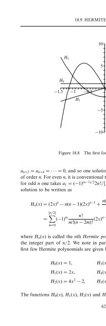
- Page 1306: SPECIAL FUNCTIONSwhere, in the seco
- Page 1312: 18.9 HERMITE FUNCTIONS◮Show thatI
- Page 1316: 18.10 HYPERGEOMETRIC FUNCTIONSby ma
- Page 1320: 18.10 HYPERGEOMETRIC FUNCTIONSF(a,
- Page 1324: 18.11 CONFLUENT HYPERGEOMETRIC FUNC
- Page 1328: 18.12 THE GAMMA FUNCTION AND RELATE
- Page 1332: 18.12 THE GAMMA FUNCTION AND RELATE
- Page 1336: 18.12 THE GAMMA FUNCTION AND RELATE
- Page 1340: 18.13 EXERCISES√√Y0 0 = 1, Y 04
- Page 1344: 18.13 EXERCISES[ You will find it c
- Page 1348: 18.13 EXERCISES(a) use their series
- Page 1352: 18.14 HINTS AND ANSWERS18.15 (a) Sh
- Page 1356: 19.1 OPERATOR FORMALISMrepresent di
- Page 1360:
19.1 OPERATOR FORMALISMspectrum of
- Page 1364:
19.1 OPERATOR FORMALISMwhilstthatfo
- Page 1368:
19.1 OPERATOR FORMALISMdefining ser
- Page 1372:
19.2 PHYSICAL EXAMPLES OF OPERATORS
- Page 1376:
19.2 PHYSICAL EXAMPLES OF OPERATORS
- Page 1380:
19.2 PHYSICAL EXAMPLES OF OPERATORS
- Page 1384:
19.2 PHYSICAL EXAMPLES OF OPERATORS
- Page 1388:
19.2 PHYSICAL EXAMPLES OF OPERATORS
- Page 1392:
19.2 PHYSICAL EXAMPLES OF OPERATORS
- Page 1396:
19.2 PHYSICAL EXAMPLES OF OPERATORS
- Page 1400:
19.3 EXERCISESthat would involve a
- Page 1404:
19.3 EXERCISESNow evaluate the expe
- Page 1408:
20Partial differential equations:ge
- Page 1412:
20.1 IMPORTANT PARTIAL DIFFERENTIAL
- Page 1416:
20.1 IMPORTANT PARTIAL DIFFERENTIAL
- Page 1420:
20.3 GENERAL AND PARTICULAR SOLUTIO
- Page 1424:
20.3 GENERAL AND PARTICULAR SOLUTIO
- Page 1428:
20.3 GENERAL AND PARTICULAR SOLUTIO
- Page 1432:
20.3 GENERAL AND PARTICULAR SOLUTIO
- Page 1436:
20.3 GENERAL AND PARTICULAR SOLUTIO
- Page 1440:
20.3 GENERAL AND PARTICULAR SOLUTIO
- Page 1444:
20.4 THE WAVE EQUATION20.4 The wave
- Page 1448:
20.5 THE DIFFUSION EQUATIONterm is
- Page 1452:
20.5 THE DIFFUSION EQUATIONwritten
- Page 1456:
20.6 CHARACTERISTICS AND THE EXISTE
- Page 1460:
20.6 CHARACTERISTICS AND THE EXISTE
- Page 1464:
20.6 CHARACTERISTICS AND THE EXISTE
- Page 1468:
20.7 UNIQUENESS OF SOLUTIONSEquatio
- Page 1472:
20.8 EXERCISESWe also note that oft
- Page 1476:
20.8 EXERCISES20.14 Solve∂ 2 u u
- Page 1480:
20.9 HINTS AND ANSWERS20.25 The Kle
- Page 1484:
21Partial differential equations:se
- Page 1488:
21.1 SEPARATION OF VARIABLES: THE G
- Page 1492:
21.2 SUPERPOSITION OF SEPARATED SOL
- Page 1496:
21.2 SUPERPOSITION OF SEPARATED SOL
- Page 1500:
21.2 SUPERPOSITION OF SEPARATED SOL
- Page 1504:
21.2 SUPERPOSITION OF SEPARATED SOL
- Page 1508:
21.3 SEPARATION OF VARIABLES IN POL
- Page 1512:
21.3 SEPARATION OF VARIABLES IN POL
- Page 1516:
21.3 SEPARATION OF VARIABLES IN POL
- Page 1520:
21.3 SEPARATION OF VARIABLES IN POL
- Page 1524:
21.3 SEPARATION OF VARIABLES IN POL
- Page 1528:
21.3 SEPARATION OF VARIABLES IN POL
- Page 1532:
21.3 SEPARATION OF VARIABLES IN POL
- Page 1536:
21.3 SEPARATION OF VARIABLES IN POL
- Page 1540:
21.3 SEPARATION OF VARIABLES IN POL
- Page 1544:
21.3 SEPARATION OF VARIABLES IN POL
- Page 1548:
21.3 SEPARATION OF VARIABLES IN POL
- Page 1552:
21.4 INTEGRAL TRANSFORM METHODS21.4
- Page 1556:
21.4 INTEGRAL TRANSFORM METHODS◮A
- Page 1560:
21.5 INHOMOGENEOUS PROBLEMS - GREEN
- Page 1564:
21.5 INHOMOGENEOUS PROBLEMS - GREEN
- Page 1568:
21.5 INHOMOGENEOUS PROBLEMS - GREEN
- Page 1572:
21.5 INHOMOGENEOUS PROBLEMS - GREEN
- Page 1576:
21.5 INHOMOGENEOUS PROBLEMS - GREEN
- Page 1580:
21.5 INHOMOGENEOUS PROBLEMS - GREEN
- Page 1584:
21.5 INHOMOGENEOUS PROBLEMS - GREEN
- Page 1588:
21.5 INHOMOGENEOUS PROBLEMS - GREEN
- Page 1592:
21.6 EXERCISESUsing plane polar coo
- Page 1596:
21.6 EXERCISES(a) Evaluate dPl m(µ
- Page 1600:
21.6 EXERCISES21.18 A sphere of rad
- Page 1604:
21.7 HINTS AND ANSWERSin V and take
- Page 1608:
22Calculus of variationsIn chapters
- Page 1612:
22.2 SPECIAL CASESto these variatio
- Page 1616:
22.2 SPECIAL CASESydsdydxxFigure 22
- Page 1620:
22.3 SOME EXTENSIONSbzρ−ba(a) (b
- Page 1624:
22.3 SOME EXTENSIONSy(x)+η(x)∆yy
- Page 1628:
22.4 CONSTRAINED VARIATIONwhere k i
- Page 1632:
22.5 PHYSICAL VARIATIONAL PRINCIPLE
- Page 1636:
22.5 PHYSICAL VARIATIONAL PRINCIPLE
- Page 1640:
22.6 GENERAL EIGENVALUE PROBLEMScon
- Page 1644:
22.7 ESTIMATION OF EIGENVALUES AND
- Page 1648:
22.8 ADJUSTMENT OF PARAMETERSIt is
- Page 1652:
22.9 EXERCISES22.9 Exercises22.1 A
- Page 1656:
22.9 EXERCISESpath of a small test
- Page 1660:
22.10 HINTS AND ANSWERStotal energy
- Page 1664:
23Integral equationsIt is not unusu
- Page 1668:
23.3 OPERATOR NOTATION AND THE EXIS
- Page 1672:
23.4 CLOSED-FORM SOLUTIONS23.4.1 Se
- Page 1676:
23.4 CLOSED-FORM SOLUTIONS23.4.2 In
- Page 1680:
23.4 CLOSED-FORM SOLUTIONSso we can
- Page 1684:
23.5 NEUMANN SERIES23.5 Neumann ser
- Page 1688:
23.6 FREDHOLM THEORYcommon ratio λ
- Page 1692:
23.7 SCHMIDT-HILBERT THEORYLet us b
- Page 1696:
23.8 EXERCISESthus Hermitian. In or
- Page 1700:
23.8 EXERCISES(b) Obtain the eigenv
- Page 1704:
23.9 HINTS AND ANSWERS23.9 Hints an
- Page 1708:
24.1 FUNCTIONS OF A COMPLEX VARIABL
- Page 1712:
24.2 THE CAUCHY-RIEMANN RELATIONS
- Page 1716:
24.2 THE CAUCHY-RIEMANN RELATIONSSi
- Page 1720:
24.3 POWER SERIES IN A COMPLEX VARI
- Page 1724:
24.4 SOME ELEMENTARY FUNCTIONSreal-
- Page 1728:
24.5 MULTIVALUED FUNCTIONS AND BRAN
- Page 1732:
24.6 SINGULARITIES AND ZEROS OF COM
- Page 1736:
24.7 CONFORMAL TRANSFORMATIONSThus
- Page 1740:
24.7 CONFORMAL TRANSFORMATIONSpoint
- Page 1744:
24.7 CONFORMAL TRANSFORMATIONSysw 5
- Page 1748:
24.8 COMPLEX INTEGRALSyw 3 s w 3w =
- Page 1752:
24.8 COMPLEX INTEGRALSyRtyyC 1 C 2R
- Page 1756:
24.9 CAUCHY’S THEOREMnamely Cauch
- Page 1760:
24.10 CAUCHY’S INTEGRAL FORMULAyC
- Page 1764:
24.11 TAYLOR AND LAURENT SERIESFurt
- Page 1768:
24.11 TAYLOR AND LAURENT SERIESof o
- Page 1772:
24.11 TAYLOR AND LAURENT SERIESdeno
- Page 1776:
24.12 RESIDUE THEOREMSuppose the fu
- Page 1780:
24.13 DEFINITE INTEGRALS USING CONT
- Page 1784:
24.13 DEFINITE INTEGRALS USING CONT
- Page 1788:
24.13 DEFINITE INTEGRALS USING CONT
- Page 1792:
24.14 EXERCISESWe have seen that
- Page 1796:
24.14 EXERCISES24.14 Prove that, fo
- Page 1800:
25Applications of complex variables
- Page 1804:
25.1 COMPLEX POTENTIALSthe field pr
- Page 1808:
25.1 COMPLEX POTENTIALSyQxPˆnFigur
- Page 1812:
25.2 APPLICATIONS OF CONFORMAL TRAN
- Page 1816:
25.3 LOCATION OF ZEROSφ =0yπ/αz
- Page 1820:
25.3 LOCATION OF ZEROSpolynomials,
- Page 1824:
25.4 SUMMATION OF SERIES◮By consi
- Page 1828:
25.5 INVERSE LAPLACE TRANSFORMΓRΓ
- Page 1832:
25.5 INVERSE LAPLACE TRANSFORMf(x)1
- Page 1836:
25.6 STOKES’ EQUATION AND AIRY IN
- Page 1840:
25.6 STOKES’ EQUATION AND AIRY IN
- Page 1844:
25.6 STOKES’ EQUATION AND AIRY IN
- Page 1848:
25.7 WKB METHODSthere exist many re
- Page 1852:
25.7 WKB METHODSThis still requires
- Page 1856:
25.7 WKB METHODSThe precise combina
- Page 1860:
25.7 WKB METHODSfor some constant A
- Page 1864:
25.7 WKB METHODSone function and th
- Page 1868:
25.8 APPROXIMATIONS TO INTEGRALSFin
- Page 1872:
25.8 APPROXIMATIONS TO INTEGRALSFro
- Page 1876:
25.8 APPROXIMATIONS TO INTEGRALSany
- Page 1880:
25.8 APPROXIMATIONS TO INTEGRALSto
- Page 1884:
25.8 APPROXIMATIONS TO INTEGRALSwhi
- Page 1888:
25.8 APPROXIMATIONS TO INTEGRALS(a)
- Page 1892:
25.8 APPROXIMATIONS TO INTEGRALSare
- Page 1896:
25.8 APPROXIMATIONS TO INTEGRALS◮
- Page 1900:
25.9 EXERCISESimaginary z-axes, fin
- Page 1904:
25.9 EXERCISES(b) Calculate F(s) on
- Page 1908:
25.10 HINTS AND ANSWERSt = −i and
- Page 1912:
26TensorsIt may seem obvious that t
- Page 1916:
26.2 CHANGE OF BASISIn the second o
- Page 1920:
26.3 CARTESIAN TENSORSx 2x ′ 1x
- Page 1924:
26.4 FIRST- AND ZERO-ORDER CARTESIA
- Page 1928:
26.5 SECOND- AND HIGHER-ORDER CARTE
- Page 1932:
26.5 SECOND- AND HIGHER-ORDER CARTE
- Page 1936:
26.7 THE QUOTIENT LAWAn operation t
- Page 1940:
26.8 THE TENSORS δ ij AND ɛ ijkN
- Page 1944:
26.8 THE TENSORS δ ij AND ɛ ijk
- Page 1948:
26.9 ISOTROPIC TENSORSare independe
- Page 1952:
26.10 IMPROPER ROTATIONS AND PSEUDO
- Page 1956:
26.11 DUAL TENSORSformations, for w
- Page 1960:
26.12 PHYSICAL APPLICATIONS OF TENS
- Page 1964:
26.12 PHYSICAL APPLICATIONS OF TENS
- Page 1968:
26.14 NON-CARTESIAN COORDINATESThe
- Page 1972:
26.15 THE METRIC TENSORsecond-order
- Page 1976:
26.15 THE METRIC TENSORwhere we hav
- Page 1980:
26.16 GENERAL COORDINATE TRANSFORMA
- Page 1984:
26.17 RELATIVE TENSORS◮Show that
- Page 1988:
26.18 DERIVATIVES OF BASIS VECTORS
- Page 1992:
26.18 DERIVATIVES OF BASIS VECTORS
- Page 1996:
26.19 COVARIANT DIFFERENTIATIONcons
- Page 2000:
26.20 VECTOR OPERATORS IN TENSOR FO
- Page 2004:
26.20 VECTOR OPERATORS IN TENSOR FO
- Page 2008:
26.21 ABSOLUTE DERIVATIVES ALONG CU
- Page 2012:
26.23 EXERCISESWriting out the cova
- Page 2016:
26.23 EXERCISES26.10 A symmetric se
- Page 2020:
26.23 EXERCISES26.23 A fourth-order
- Page 2024:
26.24 HINTS AND ANSWERSin the (mult
- Page 2028:
27.1 ALGEBRAIC AND TRANSCENDENTAL E
- Page 2032:
27.1 ALGEBRAIC AND TRANSCENDENTAL E
- Page 2036:
27.1 ALGEBRAIC AND TRANSCENDENTAL E
- Page 2040:
27.1 ALGEBRAIC AND TRANSCENDENTAL E
- Page 2044:
27.2 CONVERGENCE OF ITERATION SCHEM
- Page 2048:
27.3 SIMULTANEOUS LINEAR EQUATIONSv
- Page 2052:
27.3 SIMULTANEOUS LINEAR EQUATIONSt
- Page 2056:
. . .. . .27.3 SIMULTANEOUS LINEAR
- Page 2060:
27.4 NUMERICAL INTEGRATION(a) (b) (
- Page 2064:
27.4 NUMERICAL INTEGRATIONThis prov
- Page 2068:
27.4 NUMERICAL INTEGRATION27.4.3 Ga
- Page 2072:
27.4 NUMERICAL INTEGRATIONso, provi
- Page 2076:
27.4 NUMERICAL INTEGRATIONfactor is
- Page 2080:
27.4 NUMERICAL INTEGRATIONhas becom
- Page 2084:
27.4 NUMERICAL INTEGRATIONwill have
- Page 2088:
27.4 NUMERICAL INTEGRATIONy = f(x)y
- Page 2092:
27.4 NUMERICAL INTEGRATIONIt will b
- Page 2096:
27.5 FINITE DIFFERENCESmany values
- Page 2100:
27.6 DIFFERENTIAL EQUATIONSx h y(ex
- Page 2104:
27.6 DIFFERENTIAL EQUATIONSbut they
- Page 2108:
27.6 DIFFERENTIAL EQUATIONSThe forw
- Page 2112:
27.6 DIFFERENTIAL EQUATIONSWe assum
- Page 2116:
27.7 HIGHER-ORDER EQUATIONSy1.00.80
- Page 2120:
27.8 PARTIAL DIFFERENTIAL EQUATIONS
- Page 2124:
27.9 EXERCISES27.9 Exercises27.1 Us
- Page 2128:
27.9 EXERCISES(b) Try to repeat the
- Page 2132:
27.9 EXERCISES27.21 Write a compute
- Page 2136:
27.10 HINTS AND ANSWERS27.27 The Sc
- Page 2140:
28Group theoryFor systems that have
- Page 2144:
28.1 GROUPS28.1.1 Definition of a g
- Page 2148:
28.1 GROUPS◮Using only the first
- Page 2152:
28.1 GROUPSLMKFigure 28.2 Reflectio
- Page 2156:
28.2 FINITE GROUPS28.2 Finite group
- Page 2160:
28.2 FINITE GROUPS(a)1 5 7 111 1 5
- Page 2164:
28.3 NON-ABELIAN GROUPSAs a first e
- Page 2168:
28.3 NON-ABELIAN GROUPSI A B C D EI
- Page 2172:
28.4 PERMUTATION GROUPSSuppose that
- Page 2176:
28.5 MAPPINGS BETWEEN GROUPS28.5 Ma
- Page 2180:
28.6 SUBGROUPS(a)I A B C D EI I A B
- Page 2184:
28.7 SUBDIVIDING A GROUP(i) the set
- Page 2188:
28.7 SUBDIVIDING A GROUPthis implie
- Page 2192:
28.7 SUBDIVIDING A GROUP• Two cos
- Page 2196:
28.7 SUBDIVIDING A GROUP(iii) In an
- Page 2200:
28.8 EXERCISES28.4 Prove that the r
- Page 2204:
28.8 EXERCISESSimilarly compute C 2
- Page 2208:
28.9 HINTS AND ANSWERS≠For Φ 4 ,
- Page 2212:
29.1 DIPOLE MOMENTS OF MOLECULESABA
- Page 2216:
29.2 CHOOSING AN APPROPRIATE FORMAL
- Page 2220:
29.2 CHOOSING AN APPROPRIATE FORMAL
- Page 2224:
29.2 CHOOSING AN APPROPRIATE FORMAL
- Page 2228:
29.3 EQUIVALENT REPRESENTATIONSresp
- Page 2232:
29.4 REDUCIBILITY OF A REPRESENTATI
- Page 2236:
29.4 REDUCIBILITY OF A REPRESENTATI
- Page 2240:
29.5 THE ORTHOGONALITY THEOREM FOR
- Page 2244:
29.6 CHARACTERS3m I A, B C, D, EA 1
- Page 2248:
29.7 COUNTING IRREPS USING CHARACTE
- Page 2252:
29.7 COUNTING IRREPS USING CHARACTE
- Page 2256:
29.7 COUNTING IRREPS USING CHARACTE
- Page 2260:
29.8 CONSTRUCTION OF A CHARACTER TA
- Page 2264:
29.10 PRODUCT REPRESENTATIONSgive a
- Page 2268:
29.11 PHYSICAL APPLICATIONS OF GROU
- Page 2272:
29.11 PHYSICAL APPLICATIONS OF GROU
- Page 2276:
29.11 PHYSICAL APPLICATIONS OF GROU
- Page 2280:
29.11 PHYSICAL APPLICATIONS OF GROU
- Page 2284:
29.12 EXERCISESas the sum of two on
- Page 2288:
29.12 EXERCISESUse this to show tha
- Page 2292:
29.13 HINTS AND ANSWERS(a) Make an
- Page 2296:
30ProbabilityAll scientists will kn
- Page 2300:
30.1 VENN DIAGRAMSA42 6 3BS15Figure
- Page 2304:
30.1 VENN DIAGRAMSgets beyond three
- Page 2308:
30.2 PROBABILITYtimes then we expec
- Page 2312:
30.2 PROBABILITYHowever, we may wri
- Page 2316:
30.2 PROBABILITYace from a pack of
- Page 2320:
30.2 PROBABILITYA 4A 3OA 1A 2BFigur
- Page 2324:
30.3 PERMUTATIONS AND COMBINATIONSW
- Page 2328:
30.3 PERMUTATIONS AND COMBINATIONSt
- Page 2332:
30.3 PERMUTATIONS AND COMBINATIONSm
- Page 2336:
30.4 RANDOM VARIABLES AND DISTRIBUT
- Page 2340:
30.4 RANDOM VARIABLES AND DISTRIBUT
- Page 2344:
30.5 PROPERTIES OF DISTRIBUTIONSIn
- Page 2348:
30.5 PROPERTIES OF DISTRIBUTIONSInt
- Page 2352:
30.5 PROPERTIES OF DISTRIBUTIONS|x
- Page 2356:
30.5 PROPERTIES OF DISTRIBUTIONSWe
- Page 2360:
30.6 FUNCTIONS OF RANDOM VARIABLESf
- Page 2364:
30.6 FUNCTIONS OF RANDOM VARIABLESY
- Page 2368:
30.6 FUNCTIONS OF RANDOM VARIABLESw
- Page 2372:
30.7 GENERATING FUNCTIONSvariance o
- Page 2376:
30.7 GENERATING FUNCTIONSand differ
- Page 2380:
30.7 GENERATING FUNCTIONSi.e. the P
- Page 2384:
30.7 GENERATING FUNCTIONSThe MGF wi
- Page 2388:
30.7 GENERATING FUNCTIONSprobabilit
- Page 2392:
30.7 GENERATING FUNCTIONSComparing
- Page 2396:
30.8 IMPORTANT DISCRETE DISTRIBUTIO
- Page 2400:
30.8 IMPORTANT DISCRETE DISTRIBUTIO
- Page 2404:
30.8 IMPORTANT DISCRETE DISTRIBUTIO
- Page 2408:
30.8 IMPORTANT DISCRETE DISTRIBUTIO
- Page 2412:
30.8 IMPORTANT DISCRETE DISTRIBUTIO
- Page 2416:
30.9 IMPORTANT CONTINUOUS DISTRIBUT
- Page 2420:
30.9 IMPORTANT CONTINUOUS DISTRIBUT
- Page 2424:
30.9 IMPORTANT CONTINUOUS DISTRIBUT
- Page 2428:
30.9 IMPORTANT CONTINUOUS DISTRIBUT
- Page 2432:
30.9 IMPORTANT CONTINUOUS DISTRIBUT
- Page 2436:
30.9 IMPORTANT CONTINUOUS DISTRIBUT
- Page 2440:
30.9 IMPORTANT CONTINUOUS DISTRIBUT
- Page 2444:
30.9 IMPORTANT CONTINUOUS DISTRIBUT
- Page 2448:
30.10 THE CENTRAL LIMIT THEOREMand
- Page 2452:
30.11 JOINT DISTRIBUTIONSconsult on
- Page 2456:
30.12 PROPERTIES OF JOINT DISTRIBUT
- Page 2460:
30.12 PROPERTIES OF JOINT DISTRIBUT
- Page 2464:
30.12 PROPERTIES OF JOINT DISTRIBUT
- Page 2468:
30.13 GENERATING FUNCTIONS FOR JOIN
- Page 2472:
30.15 IMPORTANT JOINT DISTRIBUTIONS
- Page 2476:
30.15 IMPORTANT JOINT DISTRIBUTIONS
- Page 2480:
30.16 EXERCISEStivariate Gaussian.
- Page 2484:
30.16 EXERCISES30.11 A boy is selec
- Page 2488:
30.16 EXERCISES30.18 A particle is
- Page 2492:
30.16 EXERCISESaccording to one of
- Page 2496:
30.17 HINTS AND ANSWERSconstraint
- Page 2500:
31StatisticsIn this chapter, we tur
- Page 2504:
31.2 SAMPLE STATISTICS188.7 204.7 1
- Page 2508:
31.2 SAMPLE STATISTICSand the sampl
- Page 2512:
31.2 SAMPLE STATISTICSmoments of th
- Page 2516:
31.3 ESTIMATORS AND SAMPLING DISTRI
- Page 2520:
31.3 ESTIMATORS AND SAMPLING DISTRI
- Page 2524:
31.3 ESTIMATORS AND SAMPLING DISTRI
- Page 2528:
31.3 ESTIMATORS AND SAMPLING DISTRI
- Page 2532:
31.3 ESTIMATORS AND SAMPLING DISTRI
- Page 2536:
31.3 ESTIMATORS AND SAMPLING DISTRI
- Page 2540:
31.3 ESTIMATORS AND SAMPLING DISTRI
- Page 2544:
31.4 SOME BASIC ESTIMATORSâ 2a 2(a
- Page 2548:
31.4 SOME BASIC ESTIMATORSexact exp
- Page 2552:
31.4 SOME BASIC ESTIMATORSwhere s 4
- Page 2556:
31.4 SOME BASIC ESTIMATORSthe form(
- Page 2560:
31.4 SOME BASIC ESTIMATORS(known) c
- Page 2564:
31.4 SOME BASIC ESTIMATORSSince the
- Page 2568:
31.5 MAXIMUM-LIKELIHOOD METHODSubst
- Page 2572:
31.5 MAXIMUM-LIKELIHOOD METHODL(x;
- Page 2576:
31.5 MAXIMUM-LIKELIHOOD METHOD◮In
- Page 2580:
31.5 MAXIMUM-LIKELIHOOD METHOD31.5.
- Page 2584:
31.5 MAXIMUM-LIKELIHOOD METHOD31.5.
- Page 2588:
31.5 MAXIMUM-LIKELIHOOD METHODwhere
- Page 2592:
31.5 MAXIMUM-LIKELIHOOD METHODL(x;
- Page 2596:
31.5 MAXIMUM-LIKELIHOOD METHODBy su
- Page 2600:
31.6 THE METHOD OF LEAST SQUARESThe
- Page 2604:
31.6 THE METHOD OF LEAST SQUARESwhe
- Page 2608:
31.6 THE METHOD OF LEAST SQUARESy76
- Page 2612:
31.7 HYPOTHESIS TESTINGhowever, suc
- Page 2616:
31.7 HYPOTHESIS TESTINGP (t|H 0 )α
- Page 2620:
31.7 HYPOTHESIS TESTING◮Ten indep
- Page 2624:
31.7 HYPOTHESIS TESTING◮Ten indep
- Page 2628:
31.7 HYPOTHESIS TESTINGThe sum of s
- Page 2632:
31.7 HYPOTHESIS TESTINGP (t|H 0 )0.
- Page 2636:
31.7 HYPOTHESIS TESTINGdistribution
- Page 2640:
31.7 HYPOTHESIS TESTINGλ(u)0.100.0
- Page 2644:
31.7 HYPOTHESIS TESTINGWe now turn
- Page 2648:
31.7 HYPOTHESIS TESTINGC n1 ,n 2(F)
- Page 2652:
31.7 HYPOTHESIS TESTINGIn the last
- Page 2656:
31.8 EXERCISES31.6 Prove that the s
- Page 2660:
31.8 EXERCISES31.13 A similar techn
- Page 2664:
31.9 HINTS AND ANSWERS31.9 Hints an
- Page 2668:
IndexWhere the discussion of a topi
- Page 2672:
INDEXrecurrence relations, 611-612s
- Page 2676:
INDEXcomplement, 1121probability fo
- Page 2680:
INDEXin spherical polars, 362Stoke
- Page 2684:
INDEXin cylindrical polars, 360in s
- Page 2688:
INDEXdiscontinuous functions, 420-4
- Page 2692:
INDEXnomenclature, 1102non-Abelian,
- Page 2696:
INDEXtriple, see multiple integrals
- Page 2700:
INDEXlevel lines, 905, 906Levi-Civi
- Page 2704:
INDEXMonte Carlo methods, of integr
- Page 2708:
INDEXorthogonal transformations, 93
- Page 2712:
INDEXstandard deviation σ, 1146var
- Page 2716:
INDEXwave equation, 714-716, 737, 7
- Page 2720:
INDEXsymmetric tensors, 938symmetry
- Page 2724:
INDEXvolume integrals, 396and diver