Adaptative high-gain extended Kalman filter and applications

tel-00559107, version 1 - 24 Jan 2011
5.1 Multiple Inputs, Multiple Outputs Case
The matrix ∆ has been defined such that, for all ni, i ∈ {1, ..., ny}:
This implies that for all ni, i ∈ {1, ..., ny}:
proving the first part of the lemma.
˜ni 1
bi (., u) =
θn∗−1 ˜b ni
i (., u).
� ˜ bni (˜x, u) − ˜ bni (˜z, u)� ≤Lb�x − z�,
2. The situation is simpler for the Jacobian matrix ˜ b ∗ (., u). Consider any element denoted
˜ b(i,j)(˜z). From the definition of the change of variables there exists ĩ ∈ N and ˜j ∈ N
(i.e. they can be equal to one) such that:
˜ b ∗ (i,j) (˜z) = 1
θ ĩ b∗ (i,j) (˜z)θ˜j
with ĩ ≥ ˜j (otherwise the element b∗ (i,j) = 0 because of the structure of b(x, u)). Then
proving the lemma.
�˜b ∗ (i,j) (˜z)� ≤θ˜j−ĩ ∗
�b(i,j) (˜z)� ≤ �b ∗ (i,j) (˜z)� ≤Lb.
Remark 53
When ∆ is defined in a different way, the Lipschitz constant of ˜ b isn’t Lb. The constant
actually depends on the value of θ. This leads to a inconsistent proof since Lb is used in the
definition of θ1 in the proof of Theorem 49.
When an observability form distinct from (5.1) is used, ∆ has to be redefined in such a
way that the condition (5.5) is satisfied.
We have the following set of identities:
and
(a) ∆A = θA∆, (b) A ′
∆ = θ∆A ′
,
(c) A∆−1 = θ∆−1A, (d) ∆−1A ′
= θA ′
∆−1 ,
d
F(θ,I)
(e) dt (∆) =− θ N∆, (f) d
dt
(g) ∆ −1 C ′
R −1
θ C∆−1 = ∆ −1 C ′ � 1
� ∆ −1 � = F(θ,I)
θ N∆−1 ,
θ δθRδθ
= θC ′
R−1C. � −1 C∆ −1
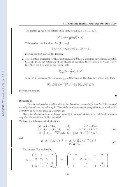
The matrix N is defined by
⎛
N1
⎜
N = ⎜ 0
⎜
⎝ .
0
N2
. ..
...
. ..
. ..
0
.
0
⎞
⎟
⎠
0 . . . 0 Nny
, Ni
⎛
n
⎜
= ⎜
⎝
∗ − ni
0
0
n
... 0
∗ − ni +1 . .
. ..
. .
. ..
.
0
0 . . . 0 n∗ ⎞
⎟
⎠
− 1
.
99
(5.6)
(5.7)