Adaptative high-gain extended Kalman filter and applications

tel-00559107, version 1 - 24 Jan 2011
2.3 Observability Normal Forms
is highly non-generic (it has co-dimension ∞, see [57]). The non-genericity of observability
is given by the two following theorems.
Theorem 9 ([38], Pg 22)
The system (Σ) has a uniform canonical flag if and only if for all x 0 ∈ X, there is a
coordinate neighborhood of x 0 , (V x 0,x), such that in those coordinates the restriction of (Σ)
to V x 0 can be written as
where ∂h
∂x1
⎧
⎪⎨
⎪⎩
y = h(x1,u)
˙x1 = f1(x1,x2,u)
˙x2 = f2(x1,x2,x3,u)
.
˙xn−1 = fn−1(x1,x2, ..., xn,u)
˙xn = fn(x1,x2, ..., xn,u)
∂fi and ∂xi+1 , i =1, ..., n − 1, never equal zero on Vx0 × Uadm.
(2.4)
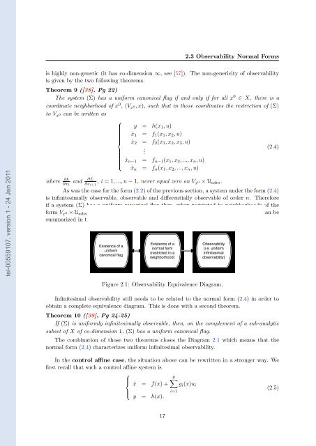
As was the case for the form (2.2) of the previous section, a system under the form (2.4)
is infinitesimally observable, observable and differentially observable of order n. Therefore
if a system (Σ) has a uniform canonical flag then when restricted to neighborhoods of the
form Vx0 × Uadm
an be
summarized in t
Existence of a
uniform
canonical flag
Existence of a
normal form
(restricted to a
neighborhood)
Observability
(i e uniform
infinitesimal
observability)
Figure 2.1: Observability Equivalence Diagram.
Infinitesimal observability still needs to be related to the normal form (2.4) in order to
obtain a complete equivalence diagram. This is done with a second theorem.
Theorem 10 ([38], Pg 24-25)
If (Σ) is uniformly infinitesimally observable, then, on the complement of a sub-analytic
subset of X of co-dimension 1, (Σ) has a uniform canonical flag.
The combination of those two theorems closes the Diagram 2.1 which means that the
normal form (2.4) characterizes uniform infinitesimal observability.
In the control affine case, the situation above can be rewritten in a stronger way. We
first recall that such a control affine system is
⎧
p�
⎪⎨
˙x = f(x)+ gi(x)ui
(2.5)
⎪⎩
i=1
y = h(x).
17