Download the entire proceedings as an Adobe PDF - Eastern Snow ...

A number of assumptions must be made in detecting snowmelt onset using this passive
microwave data. The heterogeneous and mountainous terrain within the upper Yukon River basin
most likely creates a complex Tb signal, but based largely on field observations and local weather
records, it is assumed that the majority of the land is covered with snow during the spring
transition period. In addition, since the methods focus on snowmelt events during the spring
transition from March through May, intermittent snowmelt and thaw events during the winter
months are largely ignored. It is also assumed, based on support from field data, that the events
identified with the passive microwave data as melting snow are representative of snowmelt and
not liquid precipitation events.
AMSR-E swath data were processed using the AMSR-E Swath-to-Grid Toolkit (AS2GT) in
NSIDC’s Passive Microwave Swath Data Tools (PMSDT). The data were then gridded to the
EASE-Grid Northern Hemisphere projection with a nominal resolution of 25 x 25 km 2 , the same
format and pixel resolution as the SSM/I data provided by the NSIDC. The Tb were extracted
from each channel using Interactive Data Language (IDL) code, creating a chronological time
series of all Tb observations for 2004 and 2005.
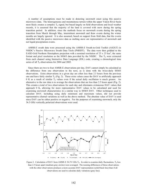
Since there are two to four AMSR-E observations per day, DAV cannot simply be calculated as
the difference from one observation to the next, as is done with the twice-daily SSM/I
observations. Extra observations in a given day are often less than 2.5 hours from the previous
one and have fairly similar Tb (Fig. 2). These extra values cause the DAV to artificially approach
0 K as a result of similar Tb values even if the actual daily oscillation is much greater. An
alternative to the raw data is to average the observations that are less than 2.5 hours apart (Fig. 2).
This creates a total of two observations for each day and eliminates extraneous DAV values that
approach 0 K, allowing for more representative DAV values to be calculated and used for
examining snowmelt characteristics in a similar way to SSM/I DAV. Other techniques used to
calculate DAV, including using daily minimum and maximum values, did not provide
representative diurnal variations as well as the above method. The absolute value of DAV is used
since DAV can be either positive or negative. For the purposes of examining snowmelt, only the
36.5 GHz vertically polarized observations were used.
Figure 2. Calculation of DAV from AMSR-E 36.5V GHz Tb. In order to examine daily fluctuations, Tb less
than 2.5 hours apart (medium gray circles) were averaged. The running differences of these observations
with the other observations produces a more accurate DAV representation (solid black line) than if all
observations are used to calculate daily variations (gray line).
142