Download the entire proceedings as an Adobe PDF - Eastern Snow ...

Following previous research by Goodison and Walker (1995) and Derksen et al. (2002, 2003b),
remotely sensed SWE estimates were compared to ground SWE measurements. The remotely
sensed estimates found to be within ±20 mm (the previously determined accuracy of the MSC
SWE algorithm) of ground measurements were considered as equivalent. SWE estimates found
not to be within the ±20 mm threshold were considered as anomalous.
Statistical Comparison Tests
Z-tests were performed between the results of the Snow-Only and Actual-Conditions data sets to
determine if there were significant differences in algorithm performance between the two groundtruth
representations. Linear regression models were developed between the remote sensing data
(as the dependant variables) and the ground observations from the coincident sampling sites (as
the independent variables).
The linear regression outputs were interpreted following the systematic procedure proposed by
Gupta (2000) (Figure 2). The significance of the model fit is analyzed. The model significance
explains the deviations of the dependent variables (eg. the SWE estimates and TB). We used a
model significance of 0.10 (90% confidence level) as the cutoff for model acceptance. Models
with levels below the 90% confidence level were removed from further analysis.
The next step in interpreting the regression output is to analyze the Adjusted R 2 value from the
model summary. This value is sensitive to the addition of irrelevant variables, and is a measure of
the proportion of the variance in the dependent variables that are explained by the variations of the
independent variables. For example, an Adjusted R 2 value of 0.500 suggests that 50% of the
variance in a SWE estimate is explained by the variation in the ground-truth measurements.
The third interpretation step involves identifying the reliability of the individual coefficients for
the independent variables. The Beta values included in the coefficients output indicate the
predicted coefficients for the model along with their standard errors and significances. Similar to
the significance of the model fit, if a coefficient results in a significance value above 0.10, then it
can be concluded that the independent variable is not significant at a 90% level of confidence.
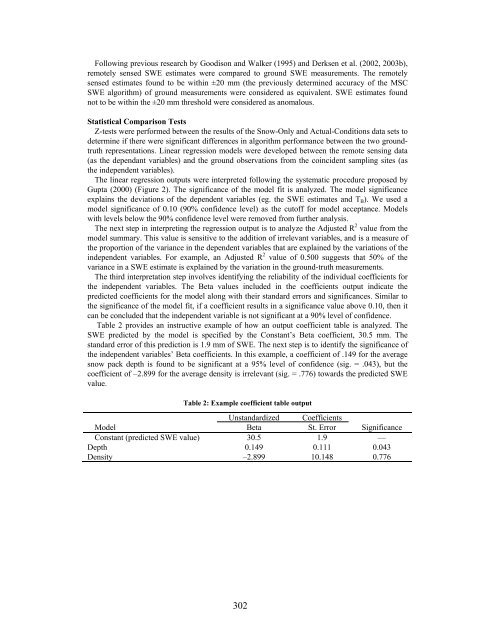
Table 2 provides an instructive example of how an output coefficient table is analyzed. The
SWE predicted by the model is specified by the Constant’s Beta coefficient, 30.5 mm. The
standard error of this prediction is 1.9 mm of SWE. The next step is to identify the significance of
the independent variables’ Beta coefficients. In this example, a coefficient of .149 for the average
snow pack depth is found to be significant at a 95% level of confidence (sig. = .043), but the
coefficient of –2.899 for the average density is irrelevant (sig. = .776) towards the predicted SWE
value.
Table 2: Example coefficient table output
Unstandardized Coefficients
Model
Beta
St. Error Significance
Constant (predicted SWE value) 30.5 1.9 —
Depth 0.149 0.111 0.043
Density –2.899 10.148 0.776
302