Download the entire proceedings as an Adobe PDF - Eastern Snow ...
Download the entire proceedings as an Adobe PDF - Eastern Snow ...
Download the entire proceedings as an Adobe PDF - Eastern Snow ...

You also want an ePaper? Increase the reach of your titles
YUMPU automatically turns print PDFs into web optimized ePapers that Google loves.
161<br />
63 rd EASTERN SNOW CONFERENCE<br />
Newark, Delaware USA 2006<br />
The left scatter plots representing <strong>the</strong> complete dat<strong>as</strong>et <strong>an</strong>d <strong>the</strong> right ones are modified by<br />
eliminating <strong>the</strong> backscattering ratio higher th<strong>an</strong> zero since only few percentage points are points<br />
have backscattering values higher th<strong>an</strong> zero. This could be <strong>the</strong> effect urb<strong>an</strong> are<strong>as</strong> that have high<br />
backscattering. The new scatter plots are shown in Figure 9. These scatter plots clearly show<br />
where SWE is in <strong>the</strong> r<strong>an</strong>ge of 10mm to 60mm <strong>the</strong> backscattering r<strong>an</strong>ge is very large. Also, <strong>the</strong><br />
backscattering r<strong>an</strong>ge between two years (2004 <strong>an</strong>d 2006) is very different. This indicates that<br />
developing a model to estimate SWE using backscattering ratio is very difficult. A solution for<br />
this problem is modifying <strong>the</strong> model for each year.<br />
Low Resolution Active QuikSCAT <strong>an</strong>d P<strong>as</strong>sive SSM/I<br />
A. Evaluation of using NDVI <strong>an</strong>d QuikSCAT in SWE estimation<br />
A feed forward backpropagation neural network model with 2 hidden layers, 20 neurons each<br />
layer, w<strong>as</strong> developed. The output of <strong>the</strong> model consists of ground truth SWE data from NOHRSC.<br />
In order to evaluate <strong>the</strong> effect SWE on various microwave ch<strong>an</strong>nels different combination of<br />
inputs were used. First, <strong>the</strong> input consisted four of SSM/I ch<strong>an</strong>nels (19V, 19H, 37V, <strong>an</strong>d 37H). Then,<br />
NDVI <strong>an</strong>d SSM/I were introduced <strong>as</strong> <strong>the</strong> input to <strong>the</strong> model. Finally, QuikSCAT-ku along with<br />
SSM/I <strong>an</strong>d NDVI were used <strong>as</strong> <strong>the</strong> input. For all above approaches <strong>the</strong> model w<strong>as</strong> validated by a<br />
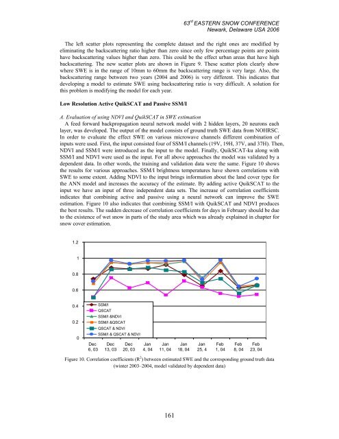
dependent data. In o<strong>the</strong>r words, <strong>the</strong> training <strong>an</strong>d validation data were <strong>the</strong> same. Figure 10 shows<br />
<strong>the</strong> results for various approaches. SSM/I brightness temperatures have shown correlations with<br />
SWE to some extent. Adding NDVI to <strong>the</strong> input brings information about <strong>the</strong> l<strong>an</strong>d cover type for<br />
<strong>the</strong> ANN model <strong>an</strong>d incre<strong>as</strong>es <strong>the</strong> accuracy of <strong>the</strong> estimate. By adding active QuikSCAT to <strong>the</strong><br />
input we have <strong>an</strong> input of three independent data sets. The incre<strong>as</strong>e of correlation coefficients<br />
indicates that combining active <strong>an</strong>d p<strong>as</strong>sive using a neural network c<strong>an</strong> improve <strong>the</strong> SWE<br />
estimation. Figure 10 also indicates that combining SSM/I with QuikSCAT <strong>an</strong>d NDVI produces<br />
<strong>the</strong> best results. The sudden decre<strong>as</strong>e of correlation coefficients for days in February should be due<br />
to <strong>the</strong> existence of wet snow in parts of <strong>the</strong> study area which w<strong>as</strong> already explained in chapter for<br />
snow cover estimation.<br />
1.2<br />
1<br />
0.8<br />
0.6<br />
0.4<br />
0.2<br />
0<br />
Dec<br />
6, 03<br />
SSM/I<br />
QSCAT<br />
SSM/I &NDVI<br />
SSM/I &QSCAT<br />
QSCAT & NDVI<br />
SSM/I & QSCAT & NDVI<br />
Dec<br />
13, 03<br />
Dec<br />
20, 03<br />
J<strong>an</strong><br />
4, 04<br />
J<strong>an</strong><br />
11, 04<br />
J<strong>an</strong><br />
18, 04<br />
J<strong>an</strong><br />
25, 4<br />
Feb<br />
1, 04<br />
Feb<br />
8, 04<br />
Feb<br />
23, 04<br />
Figure 10. Correlation coefficients (R 2 ) between estimated SWE <strong>an</strong>d <strong>the</strong> corresponding ground truth data<br />
(winter 2003–2004, model validated by dependent data)