Download the entire proceedings as an Adobe PDF - Eastern Snow ...

each other; and, they both decrease at greater rates than under the COMMIT scenario. For all
models under the SRESA1B and SRESA2 scenarios, SCE decreases at a greater rate during the
twenty first century than during the twentieth century. In contrast, under the COMMIT scenario,
while some models do have weak but significant decreasing trends in SCE, in no model does SCE
decrease at a greater rate during the twenty first century than during the twentieth century. The
differences in responses are not proportional to the differences in forcing under these scenarios,
indicating that non-linear dynamics are influencing the snow cover.
Discussion and conclusions Significant between-model variability is found in all comparisons
of GCM snow simulations: e.g. the range of simulated snow mass of North America by AMIP-2
AGCMs is ±50% of the estimated value. When using a GCM to evaluate potential changes in
regional to continental scale hydrological variations one must exercise caution. However, the
median result from all models tends to do a reasonably good job compared to observations. Thus,
perhaps a “superensemble” of models, when numerous simulations from different models are
combined, may be an effective method. Preliminary evaluations of AOGCMs suggest that:
decadal scale variability is associated with internal climatic variations and not with external
forcings in these models (whether that is true in the real climate system is unknown); and,
decreases in snow extent are expected under realistic scenarios of future emissions, although the
precise response of the snow cover to possible future climate variations may be non linear.
Figure 3. Nine-year running mean of twentieth century January NA-SCE for 11 IPCC-AR4 ensemblemean
model simulations and for reconstructions of observed variations. NA-SCE is defined as the
fraction of the land area from 20° N - 90°N and 190° E - 340° E covered with snow. The legend shows
the model number, which corresponds to model numbers and ensemble sizes shown in Table 2; “B” and
“F” correspond to Brown (2000) and Frei et al. (1999), respectively. Figure adapted from Frei and Gong
(2005).
Fractional Snow Covered Area
0.9
0.85
0.8
0.75
0.7
0.65
0.6
0.55
MRI-CGCM2.3.2
0.5
1900 1950 2000
Year
2050 2100
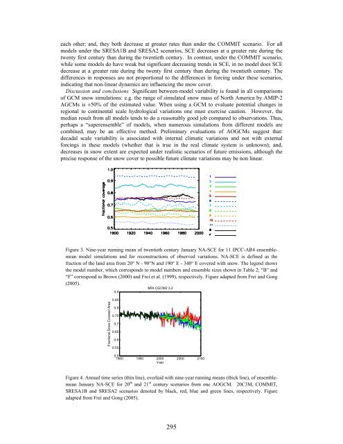
Figure 4. Annual time series (thin line), overlaid with nine-year running means (thick line), of ensemblemean
January NA-SCE for 20 th and 21 st century scenarios from one AOGCM. 20C3M, COMMIT,
SRESA1B and SRESA2 scenarios denoted by black, red, blue and green lines, respectively. Figure
adapted from Frei and Gong (2005).
295