a variacional del estado de transición a la - Páxinas persoais - USC ...

More documents

Recommendations

Info

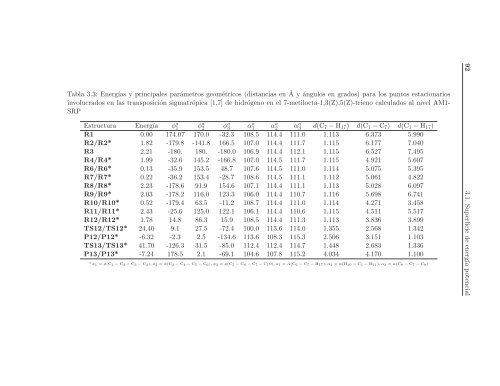
Tabla 3.3: Energías y principales parámetros geométricos (distancias en Å y ángulos en grados) para los puntos estacionariosinvolucrados en las transposición sigmatrópica [1,7] de hidrógeno en el 7-metilocta-1,3(Z),5(Z)-trieno calculados al nivel AM1-SRPEstructura Energía φ a 1 φ a 2 φ a 3 α1 a α2 a α3 a d(C 7 − H 17 ) d(C 1 − C 7 ) d(C 1 − H 17 )R1 0.00 174.07 170.0 -32.3 108.5 114.4 111.0 1.113 6.373 5.990R2/R2* 1.82 -179.8 -141.8 166.5 107.0 114.4 111.7 1.115 6.177 7.040R3 2.21 -180. 180. -180.0 106.9 114.4 112.1 1.115 6.527 7.495R4/R4* 1.99 -32.6 145.2 -166.8 107.0 114.5 111.7 1.115 4.921 5.607R6/R6* 0.13 -35.9 153.5 48.7 107.6 114.5 111.0 1.114 5.075 5.395R7/R7* 0.22 -36.2 153.4 -28.7 108.6 114.5 111.1 1.112 5.061 4.822R8/R8* 2.23 -178.6 91.9 154.6 107.1 114.4 111.1 1.113 5.028 6.097R9/R9* 2.03 -178.2 116.0 123.3 106.0 114.4 110.7 1.116 5.698 6.741R10/R10* 0.52 -179.4 63.5 -11.2 108.7 114.4 111.0 1.114 4.271 3.458R11/R11* 2.43 -25.6 125.0 122.1 106.1 114.4 110.6 1.115 4.511 5.517R12/R12* 1.78 14.8 86.3 15.9 108.5 114.4 111.3 1.113 3.836 3.899TS12/TS12* 24.40 9.1 27.5 -72.4 100.0 113.6 114.0 1.355 2.568 1.342P12/P12* -6.32 -2.3 2.5 -134.6 113.6 108.3 115.3 2.506 3.151 1.103TS13/TS13* 41.70 -126.3 31.5 -85.0 112.4 112.4 114.7 1.448 2.683 1.336P13/P13* -7.24 178.5 2.1 -69.1 104.6 107.8 115.2 4.034 4.170 1.100a φ1 = φ(C 1 − C 2 − C 3 − C 4 ), φ 2 = φ(C 3 − C 4 − C 5 − C 6 ), φ 3 = φ(C 5 − C 6 − C 7 − C 1 0), α 1 = α(C 6 − C 7 − H 17 ), α 2 = α(H 10 − C 1 − H 11 ), α 3 = α(C 8 − C 7 − C 9 )92 3.1. Superficie de energía potencial
3. Resultados y discusión 933.2. Cálculos de dinámica directaPara llevar a cabo simulaciones de las reacciones químicas se necesita informaciónacerca de la superficie de energía potencial del sistema que es objeto deestudio. La superficie de energía potencial se puede obtener como una funciónanalítica ajustada total o parcialmente a energías calculadas mediante métodosteóricos de la estructura electrónica o a propiedades empíricas ajustables.Sin embargo, con la actual potencia de cálculo es posible usar directamente lasteorías de la estructura electrónica en las simulaciones, prescindiendo de lasenergías de potencial analíticas o empíricas, es decir, que la energía potencialy sus derivadas se calculan “al vuelo”. Este tipo particular de simulaciones basadasen la aproximación de Born-Oppenheimer se denominan, simulacionesde dinámica directa Born-Oppenheimer.En la sección 2.4 de esta memoria se presenta la teoría variacional delestado de transición. Esta teoría requiere cierta información de la superficiede energía potencial, que puede ser calculada al vuelo. Este es el método quehemos utilizado para obtener las constantes de velocidad del desplazamientosigmatrópico [1,7] de hidrógeno en el 7-metilocta-1,3(Z),5(Z)-trieno .3.2.1. Detalles computacionalesLa superficie de energía potencial se ha obtenido con el programaMOPAC [65] , mientras que para el cálculo de las constantes de velocidad hemosutilizado el programa desarrollado en el grupo del Profesor D. G. Truhlar,llamado POLYRATE [66] .La teoría variacional del estado de transición requiere, al menos, el cálculodel camino de mínima energía para obtener las constantes velocidad canónicasvariacionales k CVT/tun . En el caso de que, lo que se desee es evaluar elefecto túnel de gran curvatura, es necesario calcular una región más ampliade la superficie de energía potencial. En cálculos de dinámica directa el programaPOLYRATE necesita valores de la superficie de energía potencial y susderivadas en estas regiones, concretamente en determinados puntos de las mismas.El programa de la estructura electrónica, MOPAC, debe calcular parala geometría nuclear correspondiente a esos puntos, la energía potencial y endeterminados casos el gradiente y la matriz de constantes de fuerza. Un tercerprograma debe servir de enlace entre ambos programas.A pesar de que el grupo de D. G. Truhlar desarrolló una interfaz de unión[65] J. J. P. Stewart, “MOPAC: A semiempirical molecular orbital program,” Journal ofComputer-Aided Molecular Design, vol. 4, no. 1, pp. 1–103, 1990.[66] J. C. Corchado, Y.-Y. Chuang, P. L. Fast, W.-P. Hu, Y.-P. Liu, G. C. Lynch, K. A.Nguyen, C. F. Jackels, A. Fernandez Ramos, B. A. Ellingson, B. J. Lynch, V. S. Melissas,J. Villà, I. Rossi, E. L. Coitiño, J. Pu, T. V. Albu, R. Steckler, B. C. Garrett, A. D.Isaacson, and D. G. Truhlar , “POLYRATE 9.7: Computer Program for the Calculationof Chemical Reaction Rates for Polyatomics, version 9.3.1.” Department of Chemistryand Supercomputing Institute University of Minnesota, Minneapolis, MN, June 2005.
Page 5:
VANTONIO FEZNÁNDEZ RAMOS Y SAULO A
Page 9 and 10:
Índice general1. Introducción y o
Page 12 and 13:
XIIÍNDICE DE FIGURAS3.4. Confórme
Page 15 and 16:
Capítulo 1Introducción y objetivo
Page 17 and 18:
1. Introducción y objetivos 3su ef
Page 19 and 20:
1. Introducción y objetivos 5Tabla
Page 21 and 22:
1. Introducción y objetivos 7algun
Page 23 and 24:
1. Introducción y objetivos 91.3.
Page 25 and 26:
1. Introducción y objetivos 11Tabl
Page 27 and 28:
1. Introducción y objetivos 13la p
Page 29 and 30:
1. Introducción y objetivos 15C 8
Page 31 and 32:
1. Introducción y objetivos 17Tabl
Page 33 and 34:
1. Introducción y objetivos 19C 8
Page 35 and 36:
1. Introducción y objetivos 21Figu
Page 37 and 38:
1. Introducción y objetivos 23medi
Page 39 and 40:
Capítulo 2Métodos teóricosPara a
Page 41 and 42:
2. Métodos teóricos 27Sin embargo
Page 43 and 44:
2. Métodos teóricos 29mínimo. Mi
Page 45 and 46:
2. Métodos teóricos 31podrán omi
Page 47 and 48:
2. Métodos teóricos 33Para poder
Page 49 and 50:
2. Métodos teóricos 35esférica d
Page 51 and 52:
2. Métodos teóricos 37recibe el n
Page 53 and 54:
2. Métodos teóricos 39Las integra
Page 55 and 56: 2. Métodos teóricos 41electrón l
Page 57 and 58: 2. Métodos teóricos 43son de áto
Page 59 and 60: 2. Métodos teóricos 45e INDO. Sin
Page 61 and 62: 2. Métodos teóricos 47centros y c
Page 63 and 64: 2. Métodos teóricos 492.3.3. Mét
Page 65 and 66: 2. Métodos teóricos 51cierto tama
Page 67 and 68: 2. Métodos teóricos 53Teorema var
Page 69 and 70: 2. Métodos teóricos 55el funciona
Page 71 and 72: 2. Métodos teóricos 57• Por úl
Page 73 and 74: 2. Métodos teóricos 59este nivel
Page 75 and 76: 2. Métodos teóricos 61transición
Page 77 and 78: 2. Métodos teóricos 63generalizad
Page 79 and 80: 2. Métodos teóricos 65expresión
Page 81 and 82: 2. Métodos teóricos 67(o 2) rotac
Page 83 and 84: 2. Métodos teóricos 69partición
Page 85 and 86: 2. Métodos teóricos 71en un incre
Page 87: 2. Métodos teóricos 73La segunda
Page 90 and 91: 76 3.1. Superficie de energía pote
Page 98 and 99: Tabla 3.2: Energías en kcal/mol y
Page 104 and 105: Figura 3.9: Estructuras conformacio
Page 108 and 109: 94 3.2. Cálculos de dinámica dire
Page 114 and 115: 100 3.2. Cálculos de dinámica dir
Page 117 and 118: Apéndice AMétodo simplex descende
Page 119: A. Método simplex descendente mult
Page 122 and 123: 108el que se encuentra en favor de
Page 124 and 125: 110 C.1. MORATE2end programCsubrout
Page 126 and 127: 112 C.1. MORATE2if (i.eq.icurt.or.i
Page 128 and 129: 114 C.2. CONFORATE& ,wts(nconfs,nfr
Page 130 and 131: 116 C.2. CONFORATEC TSif (nat_ts.gt
Page 132 and 133: 118 C.2. CONFORATECCCCif (iop6.eq.1
Page 134 and 135: 120 C.2. CONFORATEakp_vtst(n,i)=ct(
Page 136 and 137: 122 C.2. CONFORATECCwrite(6,30) tem
Page 138 and 139: 124 C.2. CONFORATEC Compute traslat
Page 140 and 141: 126 C.2. CONFORATEC Read input data
Page 142 and 143: 128 C.2. CONFORATECCCCenddoelsewrit
Page 144 and 145: 130 C.2. CONFORATEstop1011 write(6,
Page 146 and 147: 132 C.2. CONFORATElin=0C write(6,*)
Page 148 and 149: 134 C.2. CONFORATE& ,numsta,numstb,
Page 150 and 151: 136 C.2. CONFORATEwrite(6,33) (dmir
Page 152 and 153: 138 C.2. CONFORATEendC Compute the
Page 154 and 155: 140 C.2. CONFORATEC Full F matrixdo
Page 156 and 157:
142 C.2. CONFORATE* NAGOYA UNIVERSI
Page 158 and 159:
144 C.2. CONFORATE* * * * * * * * *
Page 160 and 161:
146 C.2. CONFORATEDO 400 J=1,N400 V
Page 162 and 163:
148 C.2. CONFORATE298. 63.0843 # Co
Page 165 and 166:
Bibliografía[1] C. Funk, “On the
Page 167 and 168:
BIBLIOGRAFÍA 153[24] A. Verloop, A
Page 169 and 170:
BIBLIOGRAFÍA 155[47] D. Hartree,
Page 171:
BIBLIOGRAFÍA 157G. Liu, A. Liashen
show all

a variacional del estado de transición a la - Páxinas persoais - USC ...

You also want an ePaper? Increase the reach of your titles

Delete template?

Save as template?