64 2.4. Dinámica químicael método <strong>de</strong> Page-McIver. Todos ellos parten <strong>de</strong> <strong>la</strong> geometría <strong><strong>de</strong>l</strong> <strong>estado</strong> <strong>de</strong><strong>transición</strong>, y a excepción <strong><strong>de</strong>l</strong> método <strong>de</strong> Page-McIver, que calcu<strong>la</strong> <strong>de</strong>rivadas<strong>de</strong> or<strong>de</strong>n superior en el <strong>estado</strong> <strong>de</strong> <strong>transición</strong>, el resto utilizan el modo normal<strong>de</strong> vibración correspondiente a <strong>la</strong> coor<strong>de</strong>nada <strong>de</strong> reacción para dar el primerpaso sobre el MEP.Si se elige una superficie divisoria que sea un hiperp<strong>la</strong>no en coor<strong>de</strong>nadasrectilíneas ortogonales al MEP, <strong>la</strong> dirección <strong><strong>de</strong>l</strong> gradiente a lo <strong>la</strong>rgo <strong><strong>de</strong>l</strong> MEPcoinci<strong>de</strong> con <strong>la</strong> dirección a lo <strong>la</strong>rgo el vector normal ˆn. Por lo tanto en estecaso, <strong>la</strong> superficie divisoria <strong>de</strong>pen<strong>de</strong> so<strong>la</strong>mente <strong>de</strong> s, y <strong>la</strong> constante <strong>de</strong> velocidadmínima se obtiene optimizando <strong>variacional</strong>mente <strong>la</strong> localización <strong>de</strong> <strong>la</strong> superficiea lo <strong>la</strong>rgo <strong><strong>de</strong>l</strong> MEP. La coor<strong>de</strong>nada perpendicu<strong>la</strong>r a <strong>la</strong> superficie divisoria es<strong>la</strong> coor<strong>de</strong>nada <strong>de</strong> reacción, y el postu<strong>la</strong>do <strong>de</strong> que no existe recruzamientopodría ser cierto si esta coor<strong>de</strong>nada es separable <strong>de</strong> los otros 3N − 1 grados<strong>de</strong> libertad. Existe <strong>de</strong> todos modos, un algoritmo que optimiza ˆn, eliminando<strong>la</strong> restricción <strong>de</strong> que <strong>la</strong> superficie divisoria sea perpendicu<strong>la</strong>r al MEP; estealgoritmo, se <strong>de</strong>nomina RODS [62] (“reorientation of the dividing surface”) ybusca maximizar <strong>la</strong> energía libre <strong>de</strong> activación en cada punto.Para c<strong>la</strong>sificar los distintos <strong>estado</strong>s <strong>de</strong> <strong>transición</strong> generalizados se utiliza<strong>la</strong> longitud <strong><strong>de</strong>l</strong> arco,s, a lo <strong>la</strong>rgo el camino <strong>de</strong> referencia, que normalmente esel MEP. El valor s = 0 se asigna al punto <strong>de</strong> sil<strong>la</strong>, y los valores negativos opositivos correspon<strong>de</strong>n al <strong>la</strong>do <strong>de</strong> los reactivos o al <strong>de</strong> los productos, respectivamente.Cada superficie divisoria generalizada en coor<strong>de</strong>nadas rectilíneasortogonales al MEP se <strong>de</strong>signa mediante el valor <strong>de</strong> s <strong><strong>de</strong>l</strong> punto <strong><strong>de</strong>l</strong> MEP quese interseca con dicha superficie.La expresión <strong>de</strong> <strong>la</strong> constante <strong>de</strong> velocidad VTST para una superficie divisoriaque interseca al MEP en s es:kC GT = 1βhQ GTCΦ R C (T)exp[−βV MEP(s)] (2.137)don<strong>de</strong> V MEP (s) es el potencial evaluado sobre el MEP en s, y Q GTCes <strong>la</strong> función<strong>de</strong> partición <strong><strong>de</strong>l</strong> <strong>estado</strong> <strong>de</strong> <strong>transición</strong> generalizado clásica. El cero <strong>de</strong> energíapara el <strong>estado</strong> <strong>de</strong> <strong>transición</strong> generalizado se toma como el mínimo <strong>de</strong> los modosvibracionales locales ortogonales al camino <strong>de</strong> reacción en s, que es igual aV MEP (s). El valor <strong>de</strong> <strong>la</strong> constante <strong>de</strong> velocidad cuando se minimiza esta ecuación,con respeto a s, correspon<strong>de</strong> a <strong>la</strong> teoría <strong><strong>de</strong>l</strong> <strong>estado</strong> <strong>de</strong> <strong>transición</strong> canónica<strong>variacional</strong>, también <strong>de</strong>nominada simplemente teoría canónica <strong>variacional</strong> (“eninglés Canonical Variational Theory, CVT”)k CVTC= mínk GTsC (T, s) = kCGT[T, sCVTC,∗ (T) ] (2.138)don<strong>de</strong> s CVTC ,∗indica <strong>la</strong> posición óptima clásica <strong>de</strong> <strong>la</strong> superficie divisoria. La[62] J. Vil<strong>la</strong> and D. G. Truh<strong>la</strong>r, “Variational transition state theory without the minimumenergypath,” Theoretical Chemistry Accounts: Theory, Computation, and Mo<strong><strong>de</strong>l</strong>ing(Theoretica Chimica Acta), vol. 97, no. 1, pp. 317–323, 1997.
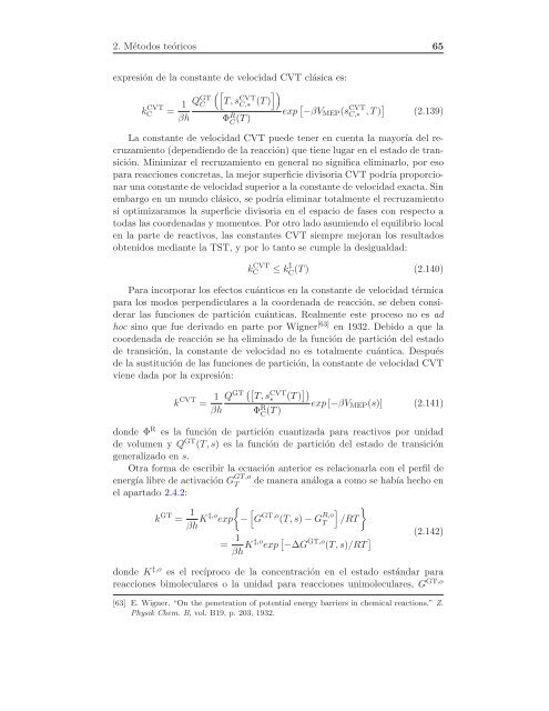
2. Métodos teóricos 65expresión <strong>de</strong> <strong>la</strong> constante <strong>de</strong> velocidad CVT clásica es:([ ])Q GTCT, s CVTC,∗ (T)k CVTC = 1βhΦ R C (T)exp [ −βV MEP (s CVTC,∗ , T) ] (2.139)La constante <strong>de</strong> velocidad CVT pue<strong>de</strong> tener en cuenta <strong>la</strong> mayoría <strong><strong>de</strong>l</strong> recruzamiento(<strong>de</strong>pendiendo <strong>de</strong> <strong>la</strong> reacción) que tiene lugar en el <strong>estado</strong> <strong>de</strong> <strong>transición</strong>.Minimizar el recruzamiento en general no significa eliminarlo, por esopara reacciones concretas, <strong>la</strong> mejor superficie divisoria CVT podría proporcionaruna constante <strong>de</strong> velocidad superior a <strong>la</strong> constante <strong>de</strong> velocidad exacta. Sinembargo en un mundo clásico, se podría eliminar totalmente el recruzamientosi optimizaramos <strong>la</strong> superficie divisoria en el espacio <strong>de</strong> fases con respecto atodas <strong>la</strong>s coor<strong>de</strong>nadas y momentos. Por otro <strong>la</strong>do asumiendo el equilibrio localen <strong>la</strong> parte <strong>de</strong> reactivos, <strong>la</strong>s constantes CVT siempre mejoran los resultadosobtenidos mediante <strong>la</strong> TST, y por lo tanto se cumple <strong>la</strong> <strong>de</strong>sigualdad:kC CVT ≤ k ‡ C(T) (2.140)Para incorporar los efectos cuánticos en <strong>la</strong> constante <strong>de</strong> velocidad térmicapara los modos perpendicu<strong>la</strong>res a <strong>la</strong> coor<strong>de</strong>nada <strong>de</strong> reacción, se <strong>de</strong>ben consi<strong>de</strong>rar<strong>la</strong>s funciones <strong>de</strong> partición cuánticas. Realmente este proceso no es adhoc sino que fue <strong>de</strong>rivado en parte por Wigner [63] en 1932. Debido a que <strong>la</strong>coor<strong>de</strong>nada <strong>de</strong> reacción se ha eliminado <strong>de</strong> <strong>la</strong> función <strong>de</strong> partición <strong><strong>de</strong>l</strong> <strong>estado</strong><strong>de</strong> <strong>transición</strong>, <strong>la</strong> constante <strong>de</strong> velocidad no es totalmente cuántica. Después<strong>de</strong> <strong>la</strong> sustitución <strong>de</strong> <strong>la</strong>s funciones <strong>de</strong> partición, <strong>la</strong> constante <strong>de</strong> velocidad CVTviene dada por <strong>la</strong> expresión:k CVT = 1 Q GT ([ T, s CVT∗ (T) ])βh Φ R C (T) exp[−βV MEP (s)] (2.141)don<strong>de</strong> Φ R es <strong>la</strong> función <strong>de</strong> partición cuantizada para reactivos por unidad<strong>de</strong> volumen y Q GT (T, s) es <strong>la</strong> función <strong>de</strong> partición <strong><strong>de</strong>l</strong> <strong>estado</strong> <strong>de</strong> <strong>transición</strong>generalizado en s.Otra forma <strong>de</strong> escribir <strong>la</strong> ecuación anterior es re<strong>la</strong>cionar<strong>la</strong> con el perfil <strong>de</strong>energía libre <strong>de</strong> activación G GT,o <strong>de</strong> manera análoga a como se había hecho enel apartado 2.4.2:k GT = 1 { [βh K‡,o exp −TG GT,o (T, s) − G R,oT] }/RT= 1βh K‡,o exp [ −∆G GT,o (T, s)/RT ] (2.142)don<strong>de</strong> K ‡,o es el recíproco <strong>de</strong> <strong>la</strong> concentración en el <strong>estado</strong> estándar parareacciones bimolecu<strong>la</strong>res o <strong>la</strong> unidad para reacciones unimolecu<strong>la</strong>res, G GT,o[63] E. Wigner, “On the penetration of potential energy barriers in chemical reactions,” Z.Physik Chem. B, vol. B19, p. 203, 1932.
- Page 5:
VANTONIO FEZNÁNDEZ RAMOS Y SAULO A
- Page 9 and 10:
Índice general1. Introducción y o
- Page 12 and 13:
XIIÍNDICE DE FIGURAS3.4. Confórme
- Page 15 and 16:
Capítulo 1Introducción y objetivo
- Page 17 and 18:
1. Introducción y objetivos 3su ef
- Page 19 and 20:
1. Introducción y objetivos 5Tabla
- Page 21 and 22:
1. Introducción y objetivos 7algun
- Page 23 and 24:
1. Introducción y objetivos 91.3.
- Page 25 and 26:
1. Introducción y objetivos 11Tabl
- Page 27 and 28: 1. Introducción y objetivos 13la p
- Page 29 and 30: 1. Introducción y objetivos 15C 8
- Page 31 and 32: 1. Introducción y objetivos 17Tabl
- Page 33 and 34: 1. Introducción y objetivos 19C 8
- Page 35 and 36: 1. Introducción y objetivos 21Figu
- Page 37 and 38: 1. Introducción y objetivos 23medi
- Page 39 and 40: Capítulo 2Métodos teóricosPara a
- Page 41 and 42: 2. Métodos teóricos 27Sin embargo
- Page 43 and 44: 2. Métodos teóricos 29mínimo. Mi
- Page 45 and 46: 2. Métodos teóricos 31podrán omi
- Page 47 and 48: 2. Métodos teóricos 33Para poder
- Page 49 and 50: 2. Métodos teóricos 35esférica d
- Page 51 and 52: 2. Métodos teóricos 37recibe el n
- Page 53 and 54: 2. Métodos teóricos 39Las integra
- Page 55 and 56: 2. Métodos teóricos 41electrón l
- Page 57 and 58: 2. Métodos teóricos 43son de áto
- Page 59 and 60: 2. Métodos teóricos 45e INDO. Sin
- Page 61 and 62: 2. Métodos teóricos 47centros y c
- Page 63 and 64: 2. Métodos teóricos 492.3.3. Mét
- Page 65 and 66: 2. Métodos teóricos 51cierto tama
- Page 67 and 68: 2. Métodos teóricos 53Teorema var
- Page 69 and 70: 2. Métodos teóricos 55el funciona
- Page 71 and 72: 2. Métodos teóricos 57• Por úl
- Page 73 and 74: 2. Métodos teóricos 59este nivel
- Page 75 and 76: 2. Métodos teóricos 61transición
- Page 77: 2. Métodos teóricos 63generalizad
- Page 81 and 82: 2. Métodos teóricos 67(o 2) rotac
- Page 83 and 84: 2. Métodos teóricos 69partición
- Page 85 and 86: 2. Métodos teóricos 71en un incre
- Page 87: 2. Métodos teóricos 73La segunda
- Page 90 and 91: 76 3.1. Superficie de energía pote
- Page 92 and 93: 78 3.1. Superficie de energía pote
- Page 94 and 95: 80 3.1. Superficie de energía pote
- Page 96 and 97: 82 3.1. Superficie de energía pote
- Page 98 and 99: Tabla 3.2: Energías en kcal/mol y
- Page 100 and 101: 86 3.1. Superficie de energía pote
- Page 102 and 103: 88 3.1. Superficie de energía pote
- Page 104 and 105: Figura 3.9: Estructuras conformacio
- Page 106 and 107: Tabla 3.3: Energías y principales
- Page 108 and 109: 94 3.2. Cálculos de dinámica dire
- Page 110 and 111: 96 3.2. Cálculos de dinámica dire
- Page 112 and 113: 98 3.2. Cálculos de dinámica dire
- Page 114 and 115: 100 3.2. Cálculos de dinámica dir
- Page 117 and 118: Apéndice AMétodo simplex descende
- Page 119: A. Método simplex descendente mult
- Page 122 and 123: 108el que se encuentra en favor de
- Page 124 and 125: 110 C.1. MORATE2end programCsubrout
- Page 126 and 127: 112 C.1. MORATE2if (i.eq.icurt.or.i
- Page 128 and 129:
114 C.2. CONFORATE& ,wts(nconfs,nfr
- Page 130 and 131:
116 C.2. CONFORATEC TSif (nat_ts.gt
- Page 132 and 133:
118 C.2. CONFORATECCCCif (iop6.eq.1
- Page 134 and 135:
120 C.2. CONFORATEakp_vtst(n,i)=ct(
- Page 136 and 137:
122 C.2. CONFORATECCwrite(6,30) tem
- Page 138 and 139:
124 C.2. CONFORATEC Compute traslat
- Page 140 and 141:
126 C.2. CONFORATEC Read input data
- Page 142 and 143:
128 C.2. CONFORATECCCCenddoelsewrit
- Page 144 and 145:
130 C.2. CONFORATEstop1011 write(6,
- Page 146 and 147:
132 C.2. CONFORATElin=0C write(6,*)
- Page 148 and 149:
134 C.2. CONFORATE& ,numsta,numstb,
- Page 150 and 151:
136 C.2. CONFORATEwrite(6,33) (dmir
- Page 152 and 153:
138 C.2. CONFORATEendC Compute the
- Page 154 and 155:
140 C.2. CONFORATEC Full F matrixdo
- Page 156 and 157:
142 C.2. CONFORATE* NAGOYA UNIVERSI
- Page 158 and 159:
144 C.2. CONFORATE* * * * * * * * *
- Page 160 and 161:
146 C.2. CONFORATEDO 400 J=1,N400 V
- Page 162 and 163:
148 C.2. CONFORATE298. 63.0843 # Co
- Page 165 and 166:
Bibliografía[1] C. Funk, “On the
- Page 167 and 168:
BIBLIOGRAFÍA 153[24] A. Verloop, A
- Page 169 and 170:
BIBLIOGRAFÍA 155[47] D. Hartree,
- Page 171:
BIBLIOGRAFÍA 157G. Liu, A. Liashen