- Page 1 and 2:
AN ABSTRACT OF A DISSERTAION AN INV
- Page 3 and 4:
coupling and interaction terms are
- Page 5 and 6:
CERTIFICATE OF APPROVAL OF DISSERTA
- Page 7 and 8:
ACKNOWLEDGEMENTS I would like to ex
- Page 9 and 10:
vi Page 2.2 Machine Design I.......
- Page 11 and 12:
viii Page 4.2.3 Self Inductances of
- Page 13 and 14:
x Page 7.3.4 f = 30 Hz and f = 95 H
- Page 15 and 16:
xii Page 10.8 D-decomposition Metho
- Page 17 and 18:
LIST OF FIGURES xiv Page Figure 1.1
- Page 19 and 20:
Figure 3.10 The simulation of the s
- Page 21 and 22:
Figure 3.34 Measured flux densities
- Page 23 and 24:
xx Page Figure 4.8 Self-inductance
- Page 25 and 26:
Figure 5.2. Simulation results for
- Page 27 and 28:
Figure 6.8. The dynamic response of
- Page 29 and 30:
Figure 7.22. Copper losses of the m
- Page 31 and 32:
Figure 8.7. The dynamic response of
- Page 33 and 34:
Figure 9.4 Steady state analysis, (
- Page 35 and 36:
Figure 9.12. The steady state wavef
- Page 37 and 38:
xxxiv Page Figure 10.16 Pole-zero m
- Page 39 and 40:
Figure 11.2 Per phase equivalent ci
- Page 41 and 42:
CHAPTER 1 INTRODUCTION AND LITERATU
- Page 43 and 44:
The last is the recently developed
- Page 45 and 46:
It should be noted that at any time
- Page 47 and 48:
A. R. Munoz and T.A. Lipo are pione
- Page 49 and 50:
has to be modified to adapt to thes
- Page 51 and 52:
circuit model of an induction machi
- Page 53 and 54:
ωr stator rotor 13 ωr rotor (a) (
- Page 55 and 56:
1.2.4 Field Analysis Method In [5.1
- Page 57 and 58:
separated dc source, etc. From the
- Page 59 and 60:
in [8.14]. In [8.15-8.17], the stud
- Page 61 and 62:
[8.22] and the total losses of the
- Page 63 and 64:
proposed. The switching frequency i
- Page 65 and 66:
The actual rotor mechanical speed i
- Page 67 and 68:
1.2.9 Induction Machine Drive---Vec
- Page 69 and 70:
stator windings were used as flux s
- Page 71 and 72:
The rotor flux can be obtained by:
- Page 73 and 74:
The basic idea of a closed loop flu
- Page 75 and 76:
estimation. It has been claimed in
- Page 77 and 78:
{ k [ ˆ* ( i iˆ ) ] ( k) [ ˆ* Im
- Page 79 and 80:
integral and a new stretch-turn ope
- Page 81 and 82:
The most recent overview paper is g
- Page 83 and 84:
CHAPTER 2 DUAL STATOR WINDING INDUC
- Page 85 and 86:
Table 2.1 Parameters of machine des
- Page 87 and 88:
A C B 2.2.2 Air Gap Flux Density X
- Page 89 and 90:
where, ω s1 and s2 respectively.
- Page 91 and 92:
There are two unknown variables in
- Page 93 and 94:
Since small machines typically have
- Page 95 and 96:
N s E = (2.18) 4. 44 fK φ 1 m Flux
- Page 97 and 98:
conduct away the heat produced in t
- Page 99 and 100:
k cs τ s = 2 2b ⎪ ⎧ ⎡ ⎤⎪
- Page 101 and 102:
are: Fts = H ts( ave) d s ( ave) =
- Page 103 and 104:
1 2 1 = H o ( ) + H o ( ) + H cr 90
- Page 105 and 106:
The skew of the stator winding is n
- Page 107 and 108:
0 bs Figure 2.5. Detailed stator sl
- Page 109 and 110:
y: The pole pitch at the mid point
- Page 111 and 112:
L lsk = L m ( α 2) ⎪⎧ ⎡sin
- Page 113 and 114:
2.3.4 Rotor Bar Resistance r b The
- Page 115 and 116:
2.3.7 Rotor Resistance Referred to
- Page 117 and 118:
Substituting δ = π into (2.97) an
- Page 119 and 120:
atio also increases. The air gap fl
- Page 121 and 122:
From (2.105-2.108), the ratio of th
- Page 123 and 124:
2.5 Conclusions In this chapter, a
- Page 125 and 126:
A recently developed dual stator wi
- Page 127 and 128:
stator winding induction machine ba
- Page 129 and 130:
∫ H ⋅ dl = ∫ J ⋅ ds = N ⋅
- Page 131 and 132:
theory itself is correct. The inacc
- Page 133 and 134:
( θ ) ⋅ g( θ, θ ) − H ( 0)
- Page 135 and 136:
where ( θ ) n A is the average of
- Page 137 and 138:
Since the definition of the mutual
- Page 139 and 140:
3Cs1 Cs1 − Cs1 − 3Cs1 6Cs1 4Cs1
- Page 141 and 142:
3.4.2 Mutual Inductances of the ABC
- Page 143 and 144:
where, ( θ ) n is the average of t
- Page 145 and 146:
1 0 α 1 − r 2π α − r 2π Fig
- Page 147 and 148:
When the skewing factor of the roto
- Page 149 and 150:
3.6 Calculation of Stator-Rotor Mut
- Page 151 and 152:
dλ v = R ⋅ i + (3.58) dt where,
- Page 153 and 154:
3.7.1.3 Stator flux linkage in ABC
- Page 155 and 156:
where, r R is the resistance matrix
- Page 157 and 158:
Only terms in equation (3.77) which
- Page 159 and 160:
119 ( ) ⎥ ⎥ ⎥ ⎥ ⎥ ⎥ ⎥
- Page 161 and 162:
−1 −1 −1 where, λ qdr = Tr L
- Page 163 and 164:
3.16 and Figure 3.17. It is found f
- Page 165 and 166:
Figure 3.11 The simulation of the d
- Page 167 and 168:
Figure 3.14 The simulation of the s
- Page 169 and 170:
Figure 3.16 Rotor bar currents duri
- Page 171 and 172:
Phase Y Figure 3.20 Air gap flux de
- Page 173 and 174:
Figure 3.24 Total air gap flux dens
- Page 175 and 176:
Figure 3.27 The air gap flux densit
- Page 177 and 178:
Figure 3.29 Air gap flux density co
- Page 179 and 180:
Figure 3.33 Air gap flux density in
- Page 181 and 182:
All the waveforms shown above are t
- Page 183 and 184:
Figure 3.39 Air gap flux density pr
- Page 185 and 186:
Figure 3.42 Normalized spectrum of
- Page 187 and 188:
Figure 3.46 Normalized spectrum of
- Page 189 and 190:
Figure 3.49 Normalized spectrum of
- Page 191 and 192:
Figure 3.53 Normalized spectrum of
- Page 193 and 194:
CHAPTER 4 FULL MODEL SIMULATION OF
- Page 195 and 196:
Substituting (3.28) and (3.29) into
- Page 197 and 198:
Figure 4.3 Self-inductance under 20
- Page 199 and 200:
Figure 4.4 Mutual inductance under
- Page 201 and 202:
that L AB = L BA , L BC = L CB and
- Page 203 and 204:
Figure 4.8 Self-inductance under 10
- Page 205 and 206:
Figure 4.10 Mutual inductance under
- Page 207 and 208:
the assumption that the rotor skew
- Page 209 and 210:
Figure 4.15 Self-inductance under 2
- Page 211 and 212:
Figure 4.17 Mutual inductance under
- Page 213 and 214:
Figure 4.19 Mutual inductance under
- Page 215 and 216:
4.4 Mutual Inductances Calculation
- Page 217 and 218:
Figure 4.24 Stator rotor mutual ind
- Page 219 and 220:
Figure 4.25 Stator rotor mutual ind
- Page 221 and 222:
varying inductances excited by four
- Page 223 and 224:
Equations similar to (4.15-4.16) we
- Page 225 and 226:
the number of poles for the winding
- Page 227 and 228:
Figure 4.29 Dynamic response of dua
- Page 229 and 230:
(a) (b) (c) (d) Figure 4.32. Normal
- Page 231 and 232:
CHAPTER 5 FIELD ANALYSIS OF DUAL ST
- Page 233 and 234:
In the analysis that follows the fu
- Page 235 and 236:
where, C s1 is the number of series
- Page 237 and 238:
θ , ∂B1 µ 0r = ⋅ J1 θ ∂θ
- Page 239 and 240:
C C = k π ⋅ d s2 s2 s2 199 (5.19
- Page 241 and 242:
the XYZ winding set is obtained by
- Page 243 and 244:
u rpi 2π ' k − jk θ −( i−1)
- Page 245 and 246:
The corresponding flux densities in
- Page 247 and 248:
The first term in equation (5.55) i
- Page 249 and 250:
The second term in (5.64) is zero u
- Page 251 and 252:
5.2.2 Torque Equation The calculati
- Page 253 and 254:
Re j( ω ) ⎧ 1t− P1θ µ 0r j(
- Page 255 and 256:
* ( ) ( ) ( ) ⎛ P1 ⋅ ⋅ ⎞ j
- Page 257 and 258:
* Since both ( ) C 2π ∫ 0 2 * Cs
- Page 259 and 260:
(A) Induced voltage in the ABC wind
- Page 261 and 262:
5.3.3 Equation of Torque Contribute
- Page 263 and 264:
winding set works as a generator, w
- Page 265 and 266:
possible for the brushless doubly-f
- Page 267 and 268:
Since the number of rotor bar is n,
- Page 269 and 270:
5.6 Computer Simulation and Experim
- Page 271 and 272:
Figure 5.2. Simulation results for
- Page 273 and 274:
5.7. Conclusions In this chapter, u
- Page 275 and 276:
good steady-state predictions and c
- Page 277 and 278:
which are superimposed some space h
- Page 279 and 280:
(a) (b) (c) Figure 6.1: Main flux s
- Page 281 and 282:
(a) (b) (c) (d) (e) Figure 6.3: Fin
- Page 283 and 284:
(a) (b) Figure 6.5: Induced air-gap
- Page 285 and 286:
Substituting (6.7) into (6.4-6.6),
- Page 287 and 288:
L L L L L L L λ + lr1 m1 ls1 m1 lr
- Page 289 and 290:
6.4 Simulation and Experimental Res
- Page 291 and 292:
Figure 6.7 . Simulation results for
- Page 293 and 294:
Figure 6.9 Experimental results for
- Page 295 and 296:
diminish the contribution of the 6-
- Page 297 and 298:
CHAPTER 7 STEADY STATE ANALYSIS OF
- Page 299 and 300:
where, L L = (7.11) si mi iqdri λq
- Page 301 and 302:
Overall efficiency of the dual stat
- Page 303 and 304:
Figure 7.2 Stator current speed cha
- Page 305 and 306:
Figure 7.6 Power factor speed chara
- Page 307 and 308:
Figure 7.9 Power factor speed chara
- Page 309 and 310:
7.3.5 f = 35Hz and f = 90 Hz abc xy
- Page 311 and 312:
Figure 7.16 Torque speed characteri
- Page 313 and 314:
this conclusion is based on the ass
- Page 315 and 316:
Figure 7.21. ω s1 vs s2 ω when to
- Page 317 and 318:
Figure 7.25 ω s1 vs s2 ω when the
- Page 319 and 320:
Figure 7.28. Copper losses of the m
- Page 321 and 322:
7.4 Conclusions Based on the steady
- Page 323 and 324:
applications and possible use as st
- Page 325 and 326:
L pλ + λ = I − = σ (8.3) ( ω
- Page 327 and 328:
espectively. The stator q and d axi
- Page 329 and 330:
* 3 * ( V I ) V Re( M I ) 3 P p = R
- Page 331 and 332:
the modulation index of the rectifi
- Page 333 and 334:
Lie derivative and relative order d
- Page 335 and 336:
The above algorithm requires that t
- Page 337 and 338:
σ = 3 1+ K ( Vqs1iqs1 + Vds1 ds1)
- Page 339 and 340:
Butterworth polynomial with the den
- Page 341 and 342:
Table 8.1 Parameters of controllers
- Page 343 and 344:
generally the case to get a good pe
- Page 345 and 346:
Table 8.2 Machine parameters for si
- Page 347 and 348:
(a) (b) (c) (d) (e) (f) (g) Figure
- Page 349 and 350:
(a) (b) (c) (d) (e) (f) (g) (h) (i)
- Page 351 and 352:
(a) (b) (c) (d) (e) (f) (g) (h) (i)
- Page 353 and 354:
CHAPTER 9 HIGH PERFORMANCE CONTROL
- Page 355 and 356:
The qd0 voltage equations of a dual
- Page 357 and 358:
317 ( ) ( ) ( ) ( ) ( ) ⎥ ⎥ ⎥
- Page 359 and 360:
If the rotor speed and the rotor fl
- Page 361 and 362:
Infeasible region (a) Vdc1 and Vdc2
- Page 363 and 364:
The influences of the saturation of
- Page 365 and 366:
Figure 9.5(a), by varying the q-axi
- Page 367 and 368:
Figure 9.5 Steady state analysis, (
- Page 369 and 370:
L1 L3 2 ( 1− K ) Vdc1 3 = ( Vqs1i
- Page 371 and 372:
If the PI controllers are used and
- Page 373 and 374:
egulation capabilities of the contr
- Page 375 and 376:
(a) (b) (c) (d) (e) (f) (g) (h) (k)
- Page 377 and 378:
(a) (b) Figure 9.11. The starting p
- Page 379 and 380:
9.6 Conclusions The high performanc
- Page 381 and 382:
induction machine are applicable to
- Page 383 and 384: In section 10.2, the fundamentals o
- Page 385 and 386: The vector control of an induction
- Page 387 and 388: possibilities for fault conditions,
- Page 389 and 390: where, where, − r r L = (10.18) (
- Page 391 and 392: qsi qsi * ( I I ) σ = K ⋅ − (1
- Page 393 and 394: In the proposed control scheme, rot
- Page 395 and 396: * ωr * ωr + + − ωr k p + ki s
- Page 397 and 398: The value of ω 0 determines the dy
- Page 399 and 400: 10.4.4 Stator D-axis Current Contro
- Page 401 and 402: (a) (b) (c) (d) (e) (f) Figure 10.4
- Page 403 and 404: The proposed control scheme has als
- Page 405 and 406: (a) (b) (c) (d) (e) (f) (g) Figure
- Page 407 and 408: 10.6 Full-order Flux Observer The c
- Page 409 and 410: while the second three-phase windin
- Page 411 and 412: L r L p ˆ λ ˆ ˆ (10.66) ri si r
- Page 413 and 414: 373 [ ] ( ) ( ) ( ) ( ) ( ) ( ) ( )
- Page 415 and 416: t 2bi ⎛ rsiLri K iL ⎞ ⎛ ri K
- Page 417 and 418: ri D i si ri ri si mi ri 2 ( K )
- Page 419 and 420: esults show that the selected obser
- Page 421 and 422: Figure 10.12 The poles of the 6-pol
- Page 423 and 424: 383 ( ) ( ) ( ) ( ) ( ) ( ) ( ) ( )
- Page 425 and 426: ⎧t s ⎨ ⎩ts 1 2 = t = t 1 2 Th
- Page 427 and 428: Figure 10.15 The poles of the machi
- Page 429 and 430: X i i = X Y = Y i i ( σ , ω) ( σ
- Page 431 and 432: this error is used as the feedback.
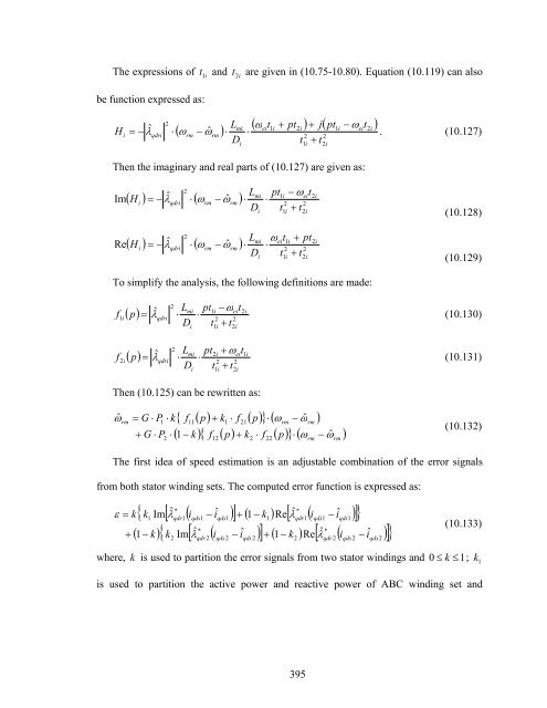
- Page 433: ˆ ω rm The output error is expres
- Page 437 and 438: 397 ( ) ( ) ( ) bi ei i bi ei i ai
- Page 439 and 440: The transfer function of rotor spee
- Page 441 and 442: (a) (b) (c) (d) Figure 10.16 Pole-z
- Page 443 and 444: Figure 10.19 Pole-zero maps with di
- Page 445 and 446: Figure 10.22 Pole-zero maps with di
- Page 447 and 448: should ensure the stability under a
- Page 449 and 450: The boundary of the speed controlle
- Page 451 and 452: 10.11 Simulation Results for Sensor
- Page 453 and 454: Figure 10.28 Speed estimation for 2
- Page 455 and 456: (a) (b) Figure 10.31 Speed estimati
- Page 457 and 458: (a) (b) (c) (d) (e) (f) Figure 10.3
- Page 459 and 460: Figure 10.34 Actual and estimated v
- Page 461 and 462: CHAPTER 11 HARDWARE IMPLEMENTATION
- Page 463 and 464: esistance for two phase windings. T
- Page 465 and 466: 11.2.3 Short Circuit Test The short
- Page 467 and 468: When the input voltages of 2-pole A
- Page 469 and 470: winding set is generating and the o
- Page 471 and 472: 11.4 Per Unit Model For the fixed p
- Page 473 and 474: 1 = 12 2 0. 0024414 The transformat
- Page 475 and 476: ase values of voltage/current. The
- Page 477 and 478: Start System configuration Initiali
- Page 479 and 480: CHAPTER 12 CONCLUSIONS AND FUTURE W
- Page 481 and 482: Using the rotating-field theory and
- Page 483 and 484: each winding have been clearly show
- Page 485 and 486:
voltages of different frequencies,
- Page 487 and 488:
REFERENCES 447
- Page 489 and 490:
[2.2]. P. C. Roberts, "A Study of B
- Page 491 and 492:
[5.3]. R. A. McMahon, P. C. Roberts
- Page 493 and 494:
[8.17]. O. Ojo, “Performance of s
- Page 495 and 496:
[10.5]. J. C. Moreira, K. T. Hung,
- Page 497 and 498:
[10.27]. M. Hinkkanen, “Analysis
- Page 499 and 500:
[10.48]. K. Lee and F. Blaabjerg,
- Page 501 and 502:
VITA Zhiqiao Wu was born in Shashi,
- Page 503:
3. Zhiqiao Wu and O. Ojo, "High Per